Time/Frequency Domain Representation of Signals

Electrical signals have both time and frequency domain representations. In the time domain, voltage or current is expressed as a function of time as illustrated in Figure 1. Most people are relatively comfortable with time domain representations of signals. Signals measured on an oscilloscope are displayed in the time domain and digital information is often conveyed by a voltage as a function of time.

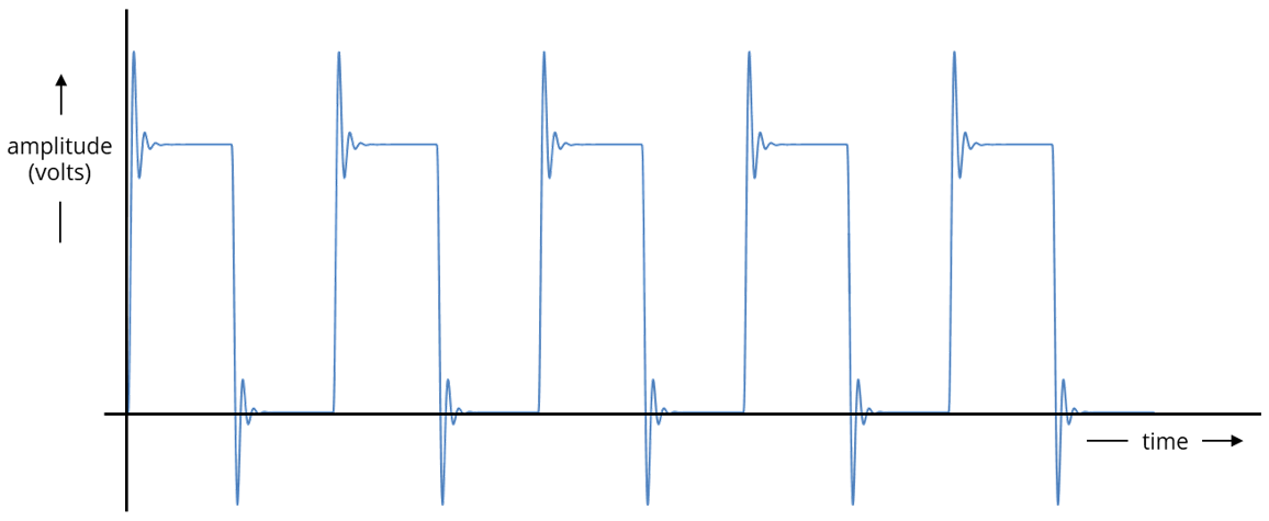
time domain digital signal with ringing

Figure 1. Time domain representation of an electrical signal.

Signals can also be represented by a magnitude and phase as a function of frequency. Signals that repeat periodically in time are represented by a line spectrum as illustrated in Figure 2. The line spectrum has a DC component at 0 Hz, a fundamental component at 1/T, and harmonics at n/T (where n is an integer). This representation is also referred to as a power spectrum because the sum of the powers in each harmonic equals the time-average power in the time-domain signal.

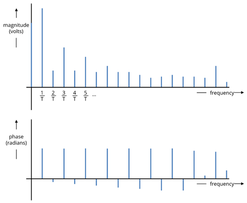
frequency domain representation of signal

Figure 2. Power spectrum of a periodic signal.

Signals that are time limited (i.e., are only non-zero for a finite time) are represented by a continuous spectrum as illustrated in Figure 3. This representation is also referred to as an energy spectrum because the sum of the integral of the energy density in this waveform over frequency equals the total energy in the time-domain signal.

energy spectrum

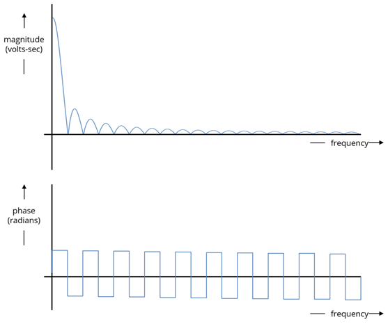
Figure 3. Energy spectrum of a time-limited (transient) signal.

Frequency domain representations are particularly useful when analyzing linear systems. EMC and signal integrity engineers must be able to work with signals represented in both the time and frequency domains. Signal sources and interference are often defined in the time domain. However, system behavior and signal transformations are more convenient and intuitive when working in the frequency domain.

Linear Systems

Linear system theory plays a key role in the engineering analysis of electrical and mechanical systems. Engineers model a wide variety of things including circuit behavior, signal propagation, coupling and radiation as linear transformations. Therefore, it is important to review exactly what we mean by a linear system so that we recognize how and when to take advantage of the powerful linear system analysis tools available to us.

Fig. 4 illustrates a system with one input, x(t), and one output, y(t)=H[x(t)]. If an input, x₁(t) produces an output y₁(t), and an input x₂(t) produces an output y₂(t), then the system is a linear system if and only if,

$a y_{1} (t) + b y_{2} (t) = H [a x_{1} (t) + b x_{2} (t)]$ (1)

where a and b are constants. In other words, scaling the input by a constant will produce an output scaled by the same constant; and combining (summing) two inputs will produce an output that is the sum of the outputs produced by the individual inputs.

linear system

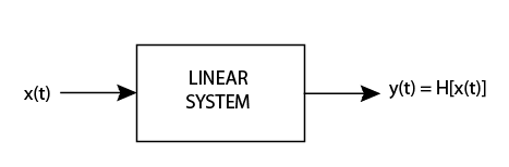
Figure 4: A linear system.

Quiz Question

Which of the following equations describes the relationship between the output y(t) and the input x(t) of a linear system?

y=5x
y(t)=0
y=8x+3
y=x²
y(t)=5t x(t)
y=sin x
y(t)=5 δ/δt [x(t)]

Of the choices above, only a, b and g are linear system transformations. y=0 is not a very interesting system, because its output is always zero, but it is linear. Simple derivative and integral operators are linear, because they satisfy the conditions in Equation (1). The remaining choices are not linear operations. Note that y=8x+3 is the equation of a straight line, but it does not describe a linear system because it has a non-zero output when there is no input.

At first, it may appear that very few real electrical or mechanical systems of interest behave this way. However, most engineering analysis depends on modeling real devices and circuits as linear systems.

Frequency Domain Analysis of Linear Systems

Linear systems have the unique property that any sinusoidal input will produce a sinusoidal output at exactly the same frequency. In other words, if the input is of the form,

$x (t) = A_{i n} \cos (ω_{0} t + φ_{i n})$ . (2)

then the output will have the form,

$y (t) = A_{o u t} \cos (ω_{0} t + φ_{o u t})$ . (3)

In general, the magnitude and phase of the sinusoidal signal may change, but the frequency must be constant. This provides us with a very powerful analysis tool for analyzing linear systems. If we represent an input signal as the sum of its components in the frequency domain, then we can express the output as a simple scaling of the magnitudes and shifting of the phases of these components.

Phasor Notation

To facilitate the analysis of linear system responses to sinusoidal inputs, it is convenient to represent signals in an abbreviated form known as phasor notation. Consider an input of the form,

$x (t) = A \cos (ω t + φ)$ . (4)

This can be represented as,

$\begin{matrix} x (t) = Re {A e^{j (ω t + φ)}} \\ = A \cdot Re {e^{j ω t} e^{j φ}} \end{matrix}$ . (5)

where Re{• } indicates the real part of a complex quantity. Recognizing that the frequency ω will be the same throughout the system, we don't need to specifically write the term e^jωt as long as we remember that it's there. The same applies to the Re{• } notation. This allows us to express a sinusoidal signal simply in terms of its magnitude and phase as,

$x = A e^{j ϕ} o r A ∠ ϕ$ . (6)

The expression in (6) is the signal in (4) expressed using phasor notation. Note that we must know the frequency of a signal in order to convert from phasor notation to the time domain representation.

Quiz Question

Write the following signals using phasor notation:

x(t) = 5 cos(ωt) volts
y(t)=5 sin(ωt) amps
z(t) = 5t sin(ωt) volts

The first signal expressed in phasor notation is simply x = 5 volts. To obtain the phasor notation for the second signal, we recognize that sin(ωt) = cos(ωt + π/2) so y = 5e^j(π/2). The third signal is not a sinusoid and therefore cannot be expressed using phasor notation.

Fourier Series

Of course many of the inputs to linear systems we would like to analyze are not sinusoidal. In this case, it is desirable to represent more arbitrary signal waveforms as a sum of sinusoidal frequency components. We then analyze each component individually and apply the concept of superposition to reconstruct the output signal.

A periodic signal can be represented as a sum of its frequency components by calculating its Fourier series coefficients. A periodic signal with period T can be written,

$x (t) = \sum_{n = - \infty}^{\infty} c_{n} e^{j n 2 π f_{0} t}$ (7a)

where

$c_{n} = \frac{1}{T} \int_{t_{0}}^{t_{0} + T} x (t) e^{- j n 2 π f_{0} t} d t$ . (7b)

If x(t) is a real time domain signal, the coefficients c_n and c_-n are complex conjugates (i.e. ) and we can rewrite Equation (7) in the form,

$\begin{array}{l} x (t) = c_{0} + \sum_{n = 1}^{\infty} (c_{n} e^{j n 2 π f_{0} t} + c_{n}^{*} e^{- j n 2 π f_{0} t}) \\ = c_{0} + \sum_{n = 1}^{\infty} (| c_{n} | e^{j n 2 π f_{0} t + ϕ_{n}} + | c_{n} | e^{- (j n 2 π f_{0} t + ϕ_{n})}) \\ = c_{0} + \sum_{n = 1}^{\infty} 2 | c_{n} | \cos (n 2 π f_{0} t + ϕ_{n}) \end{array}$ . (8)

In this form, we see that the Fourier series coefficients consist of a DC component, c₀, and positive harmonic frequencies, n2πf₀ (n = 1,2,3, …). This is a one-sided Fourier series and the coefficients, 2|c_n|, represent the peak value of each harmonic. Dividing the peak value by √2 yields the rms value. Signal harmonics measured on a spectrum analyzer or EMI test receiver are the rms values of the one-sided Fourier Series coefficients. In other words, the amplitude of each measured harmonic is √2|c_n|.

A few periodic signals and their frequency domain representations are illustrated in Figure 5. The frequency domain representation of a periodic signal is a line spectrum. It can only have non-zero values at DC, the fundamental frequency, and harmonics of the fundamental. Because periodic signals have no beginning or end, non-zero periodic signals have infinite energy but generally have finite power. The total power in the time domain signal,

$P_{t o t a l} = \frac{1}{T} \int_{t_{0}}^{t_{0} + T} x^{2} (t) d t$ . (9)

is equal to the sum of the power in each frequency domain component,

$P_{t o t a l} = \sum_{n = - \infty}^{\infty} {| c_{n} |}^{2}$ . (10)

periodic signals in time and frequency domain

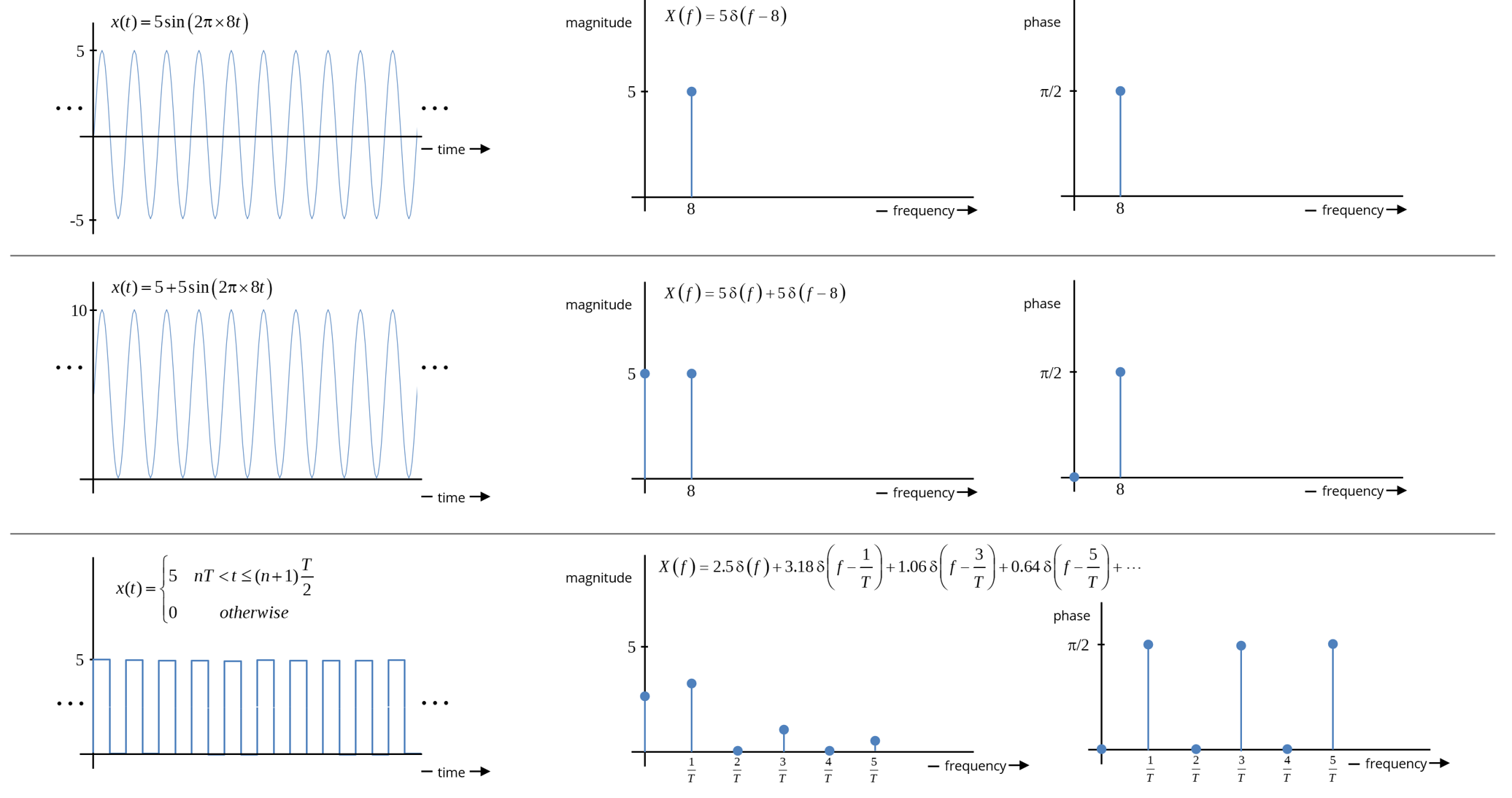
Figure 5. Periodic signals in the time and frequency domain.

Example 1: Frequency Domain Representation of a Pulse Train

Determine the frequency domain representation for the pulse train shown in Figure 6.

a rectangular pulse train

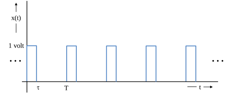
Figure 6: A pulse train.

In the time domain this signal is described by the following formula:

$x (t) = {\begin{matrix} 1 V & n T < t < n T + τ \\ 0 & o t h e r w i s e \end{matrix} n = \pm 1, \pm 2, \pm 3, \dots$ . (E1)

The coefficients of the Fourier series are then calculated using Equation (7b) as,

$\begin{array}{l} c_{n} = \frac{1}{T} \int_{0}^{T} x (t) e^{- j n 2 π f_{0} t} d t \\ = \frac{1}{T} \int_{0}^{τ} (A) e^{- j n 2 π t / T} d t \\ = \frac{A}{T} \int_{0}^{τ} e^{- j n 2 π t / T} d t \\ = \frac{A τ}{T} [\frac{\sin (\frac{n π τ}{T})}{(\frac{n π τ}{T})}] e^{- j (\frac{n π τ}{T})} \end{array}$ . (E2)

Note that as τ → 0, our time domain signal looks like an impulse train and the amplitudes of all the harmonics approach the same value. As τ → T/2, the signal becomes a square wave, and the magnitude of the harmonics becomes,

$c_{n} = \frac{A}{2} | \frac{\sin (\frac{n π}{2})}{(\frac{n π}{2})} | | e^{- j (\frac{n π}{2})} | = {\begin{matrix} \frac{A}{n π} & n = \pm 1, \pm 3, \pm 5 \dots \\ 0 & n = \pm 2, \pm 4, \pm 6 \dots \end{matrix}$ . (E3)

In this case, the amplitude of the even harmonics is zero and the odd harmonics decrease linearly with frequency (n).

Note that if we wanted to determine the amplitude of the harmonics as measured on a spectrum analyzer, we would calculate the rms amplitude of the one-sided Fourier Series coefficients,

\sqrt{2} |c_{n}| = \frac{\sqrt{2} A τ}{T} [\frac{\sin (\frac{n π τ}{T})}{(\frac{n π τ}{T})}] n = 1, 2, 3, \dots

Fourier Transform

Transient signals (i.e., signals that start and end at specific times) can also be represented in the frequency domain using the Fourier transform. The Fourier transform representation of a transient signal, x(t), is given by,

$X (f) = \int_{- \infty}^{\infty} x (t) e^{- j 2 π f t} d t$ . (11)

The inverse Fourier transform can be used to convert the frequency domain representation of a signal back to the time domain,

$x (t) = \frac{1}{2 π} \int_{- \infty}^{\infty} X (f) e^{j 2 π f t} d f$ . (12)

Two transient time domain signals and their Fourier transforms are illustrated in Figure 7.

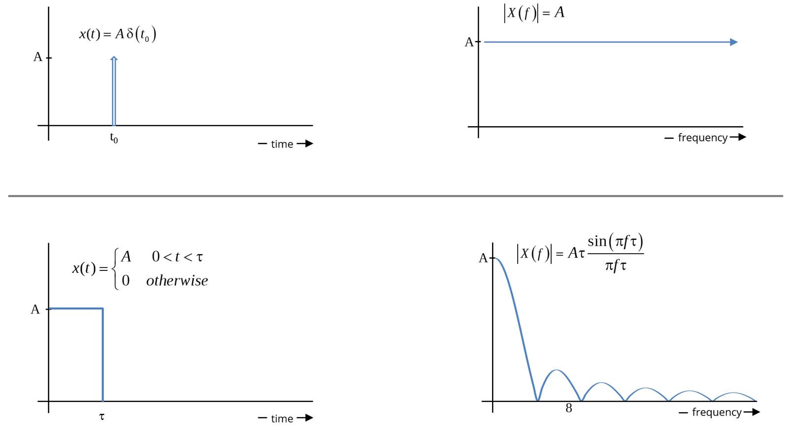
two transient signals represented in the time and frequency domains

Figure 7. Transient signals in the time and frequency domain.

Note that transient signals have zero average power (when averaged over all time), but they have finite energy. The total energy in a transient time domain signal is given by,

$E = \int_{- \infty}^{\infty} x^{2} (t) d t$ . (13)

This must equal the total energy in the frequency domain representation of the signal,

$E = {\int_{- \infty}^{\infty} | X (f) |}^{2} d f$ . (14)

Frequency Domain Representation of a Trapezoidal Signal

Let's examine the frequency domain representation of the periodic trapezoidal waveform illustrated in Figure 8. Examining the behavior of this waveform helps us to gain insight into the relationship between time and frequency domain representations in general. Also, the similarity between the trapezoidal waveform and common digital signal waveforms will be useful when we investigate EMC or signal integrity problems with digital systems.

a trapezoidal waveform

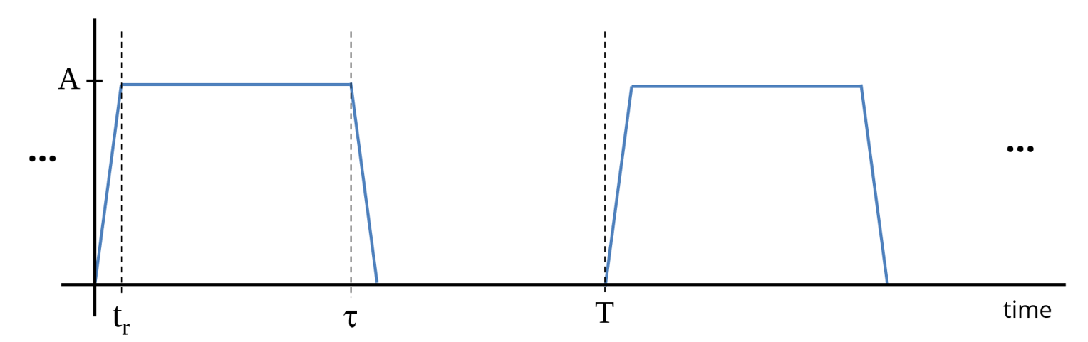
Figure 8. A trapezoidal waveform.

Using the one-sided Fourier series, Equations (7b) and (8), we can represent this signal as the sum of its frequency components [1],

$x (t) = c_{0} + \sum_{n = 1}^{\infty} 2 | c_{n} | \cos (n 2 π f_{0} t + ϕ_{n})$ . (15)

where

$2 | c_{n} | = \frac{2 A τ}{T} | \frac{\sin (\frac{n π τ}{T})}{(\frac{n π τ}{T})} | | \frac{\sin (\frac{n π t_{r}}{T})}{(\frac{n π t_{r}}{T})} |$ . (16)

Equation (16) can be derived by noting that the trapezoidal waveform in Figure 7 can be obtained by convolving the pulse train in Figure 9 with another pulse train whose pulses have a width, t_r, and an amplitude A/t_r. Convolution in the time domain is equivalent to multiplication in the frequency domain, so we can simply multiply the two frequency domain representations of these pulse trains to obtain Equation (16).

Each term, 2|c_n|, is the peak amplitude of the nth harmonic. If we assume that t_r<<T, we note that the third term is approximately equal to $\frac{\sin (small number)}{small number} \approx 1$ for the lower harmonics. If $τ = \frac{T}{2}$ (i.e., a 50% duty cycle), then the numerator of the second term is 1 for the harmonics (n = 1,3,5,…) and 0 for the even harmonics (n = 2,4,6,…). The amplitude of the lower harmonics is then inversely proportional to n (i.e., the amplitude of the lower harmonics decreases proportional to the frequency). At higher harmonics, the third term also begins to decrease proportional to frequency, so the overall amplitude of the upper harmonics decreases on average at a rate proportional to the square of the frequency. This frequency representation of a trapezoidal signal $(τ = \frac{T}{2}, t_{r} ≪ T)$ and its envelope are illustrated in Figure 9. Note that small values of τ (short duty cycles) will extend the first knee frequency, which could cause the first several harmonics to have approximately the same amplitude.

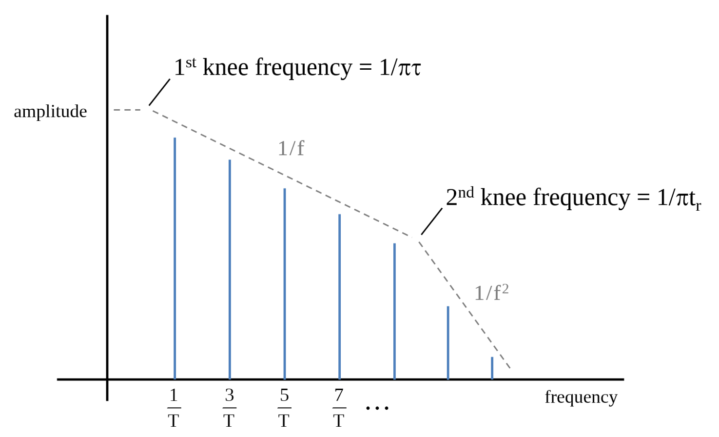
frequency domain representation of a trapezoidal signal

Figure 9: Frequency Domain representation of a trapezoidal signal

Example 2: Harmonics of a Trapezoidal Signal

The waveform shown in Figure 10 below is measured on an oscilloscope in the lab. The rise and fall times are 0.8 ns.

a.) What is the fundamental frequency?

b.) Calculate the amplitudes of the harmonics at 50 MHz, 150 MHz, 250 MHz and 1.55 GHz.

If the rise and fall times are increased to 1.6 nanoseconds, then by how many dB will the harmonics at 50 MHz, 150 MHz, 250 MHz and 550 MHz be reduced?

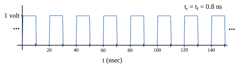
trapezoidal waveform with a period of 20 nanoseconds and a transition time of 0.8 nanoseconds. The amplitude is 1 volt.

Figure 10. Trapezoidal waveform for Example 2.

Noting that the period is 20 nsec, the fundamental frequency is easily determined to be $f_{0} = \frac{1}{T} = \frac{1}{2 \times 10^{- 8}} = 50 MHz$ . Therefore we are being asked to determine the amplitudes of the 1^st, 3^rd, 5^th and 11^th harmonics. Applying Equation (16) for n = 1,3,5 and 11 we get the amplitudes of these harmonics,

$\begin{array}{l} 2 | c_{1} | = \frac{2 (1 v)}{2} | \frac{\sin (\frac{1 π (10)}{20})}{(\frac{1 π (10)}{20})} | | \frac{\sin (\frac{1 π (0.8)}{20})}{(\frac{1 π (0.8)}{20})} | = (1 v) (0.64) (1.00) = 0.64 v \\ 2 | c_{3} | = \frac{2 (1 v)}{2} | \frac{\sin (\frac{3 π (10)}{20})}{(\frac{3 π (10)}{20})} | | \frac{\sin (\frac{3 π (0.8)}{20})}{(\frac{3 π (0.8)}{20})} | = (1 v) (0.21) (0.98) = 0.21 v \\ 2 | c_{5} | = \frac{2 (1 v)}{2} | \frac{\sin (\frac{5 π (10)}{20})}{(\frac{5 π (10)}{20})} | | \frac{\sin (\frac{5 π (0.8)}{20})}{(\frac{5 π (0.8)}{20})} | = (1 v) (0.13) (0.94) = 0.12 v \\ 2 | c_{11} | = \frac{2 (1 v)}{2} | \frac{\sin (\frac{11 π (10)}{20})}{(\frac{11 π (10)}{20})} | | \frac{\sin (\frac{11 π (0.8)}{20})}{(\frac{11 π (0.8)}{20})} | = (1 v) (0.06) (0.71) = 0.04 v \end{array}$ .

None of these harmonics are significantly affected by the risetime. They have virtually the same amplitude that they would have had if the risetime had been zero. Increasing the risetime to 1.6 ns however, significantly affects the amplitude of the upper harmonics,

$\begin{array}{l} 2 | c_{1} | = \frac{2 (1 v)}{2} | \frac{\sin (\frac{1 π (10)}{20})}{(\frac{1 π (10)}{20})} | | \frac{\sin (\frac{1 π (1.6)}{20})}{(\frac{1 π (1.6)}{20})} | = (1 v) (0.64) (.99) = 0.63 v \\ 2 | c_{3} | = \frac{2 (1 v)}{2} | \frac{\sin (\frac{3 π (10)}{20})}{(\frac{3 π (10)}{20})} | | \frac{\sin (\frac{3 π (1.6)}{20})}{(\frac{3 π (1.6)}{20})} | = (1 v) (0.21) (0.91) = 0.19 v \\ 2 | c_{5} | = \frac{2 (1 v)}{2} | \frac{\sin (\frac{5 π (10)}{20})}{(\frac{5 π (10)}{20})} | | \frac{\sin (\frac{5 π (1.6)}{20})}{(\frac{5 π (1.6)}{20})} | = (1 v) (0.13) (0.76) = 0.10 v \\ 2 | c_{11} | = \frac{2 (1 v)}{2} | \frac{\sin (\frac{11 π (10)}{20})}{(\frac{11 π (10)}{20})} | | \frac{\sin (\frac{11 π (1.6)}{20})}{(\frac{11 π (1.6)}{20})} | = (1 v) (0.06) (0.13) = 0.008 v \end{array}$ .

Doubling the risetime from 0.8 to 1.6 ns reduces the first harmonic by only $20 \log (\frac{.64}{.63}) = 0.14 dB$ . The third harmonic is reduced by $20 \log (\frac{.21}{.19}) = 0.87 dB$ . The fifth harmonic is reduced by $20 \log (\frac{.12}{.10}) = 1.6 dB$ , while the eleventh harmonic is reduced by $20 \log (\frac{0.04}{0.008}) = 14 dB$ .

Note that changing the risetime can have a significant effect on the amplitude of the upper harmonics without changing the time domain representation of the signal significantly. Radiated EMI or crosstalk problems at the upper harmonic frequencies of a digital signal can often be solved by increasing the risetime of the digital signal waveform. Generally, a risetime that is equal to 10% of a bit length or more will still produce a very good digital signal while significantly limiting the amplitude of a signal at frequencies above the 10^th harmonic.