
Transmission Lines in the Time Domain
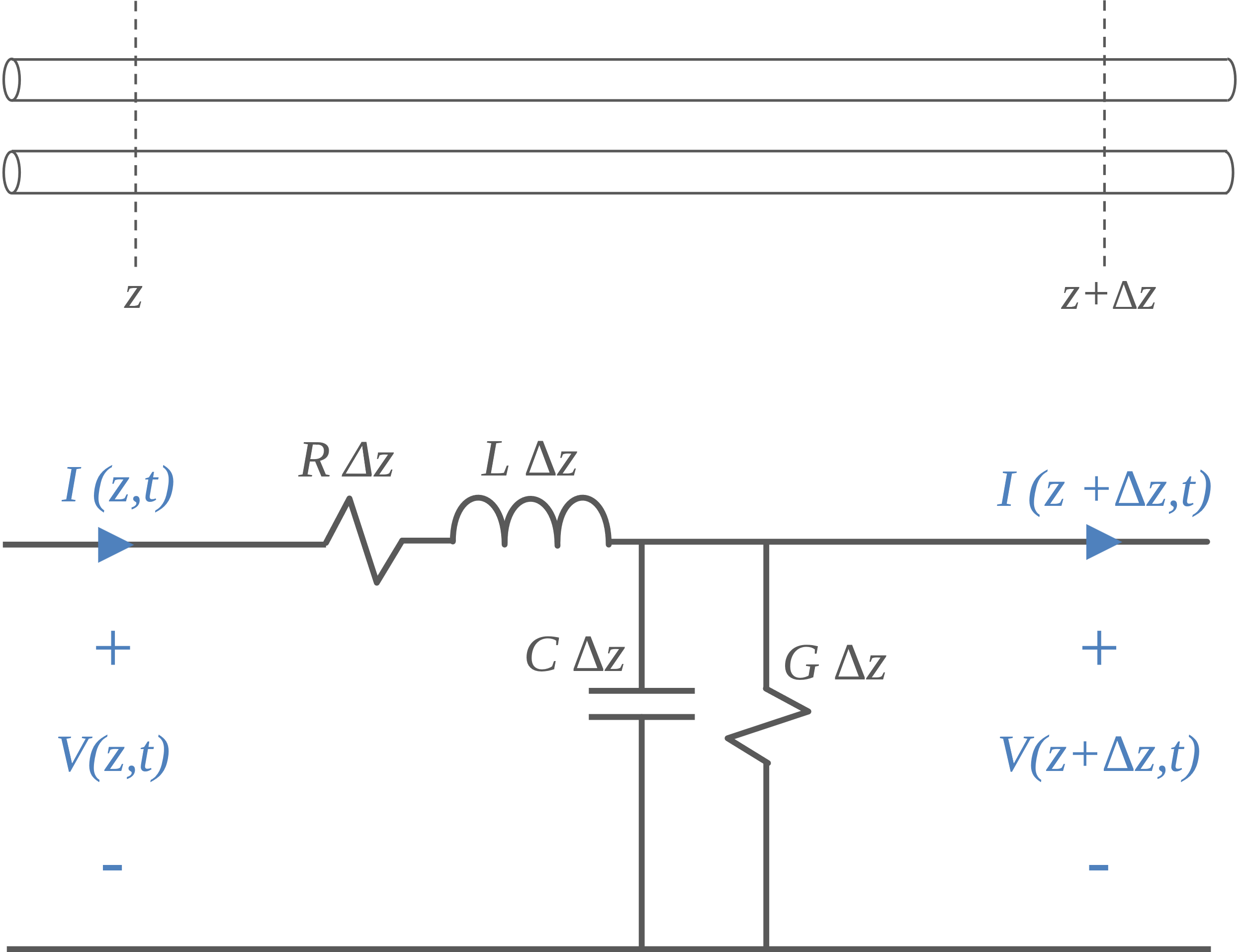
Figure 1. Equivalent circuit for a section of transmission line.
Consider the circuit representation for a single section of transmission line shown in Figure 1. V(z,t) represents the time-varying voltage at position z between the two conductors. The current on one of the conductors at position z is represented as I(z,t). Note that the currents on the two conductors of a transmission line at a given position along its length are always opposite in sign and equal in amplitude. Therefore, it is not necessary to represent the current on each conductor independently.
Applying Kirchhoff’s voltage law to the model in Figure 1, we find that the difference between the potential at position z and position z+Δz is given by,
Since Δz is electrically short, V(z+Δz, t) may be represented by its Taylor series expansion,
Neglecting the higher-order terms and substituting (2) into (1), we get
Although this is an approximation, it can be arbitrarily accurate by choosing Δz (the length of each section) to be sufficiently small.
The difference in the current at the two positions, z and z+Δz, must be equal to the current leaked through the conductance GΔz and the capacitance CΔz,
Using the Taylor series expansion as before, we obtain,
Equations (3) and (5) are coupled differential equations governing the current and voltage in transmission lines and are often referred to as the telegrapher’s equations.
Lossless Transmission Lines
If the resistance per unit length, R, and the conductance per unit length, G, of a transmission line are negligible (i.e., R ≈ G ≈ 0), then the transmission line is lossless. For a lossless line, the transmission line equations (3) and (5) reduce to,
and
Differentiating (6) with respect to z and (7) with respect to t and combining the two equations, we get an equation describing the voltage on the transmission line as a function of time and position,
Similarly, differentiating (6) with respect to t and (7) with respect to z results in an equation for the current on the transmission line,
Equations that relate a second derivative in time to a second derivative in space, like Equations (8) and (9), are wave equations. Solutions to a wave equation are linear combinations of traveling wave functions. For example, the general solution to Equation (8) can be written in the form,
where,
and F1 and F2 represent arbitrary functions. The nature of the functions F1 and F2 is determined by the source exciting the transmission line and the load terminating the transmission line.
Traveling Waves
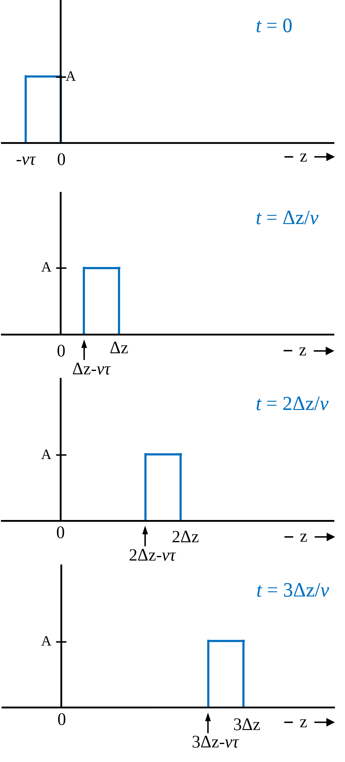
Figure 2. Pulse function propagating in the z direction.
Solutions of the form are referred to as traveling waves. Consider the rectangular pulse function given by,
This function is plotted in Figure 2 as a function of z for four different values of t. Note that as t increases, the function shifts in the z direction. The pulse effectively propagates in the z direction. The velocity of this propagation is the change in distance divided by the change in time, or
Therefore, represents a wave traveling with a velocity, v, in the z direction.
Quiz Question
What is the direction and velocity of a wave corresponding to the function, ?
In this case, as t increases, the function shifts in the -z direction with velocity, v (or the +z direction with velocity, -v). So, the general solution described in (10) is a combination of forward- and backward-traveling waves. These waves travel with the same velocity in opposite directions.
Without specifying how the transmission line is terminated, the forward- and backward-traveling waves are independent. Any number of forward and backward traveling waveforms can coexist in the line at any time.
Semi-Infinite Transmission Lines
Consider a semi-infinite line extending from z = 0 to z→∞, as illustrated in Figure 3. Before the switch is closed, there is no charge on (and therefore no voltage across) the line. At t = 0, the switch is closed, causing a voltage V0 to appear at the input to the transmission line. The voltage V0 does not appear instantly at all points along the line. Instead, a voltage wave progresses along the line. The farther a given point is from the voltage source, the later the time at which the line voltage at that point jumps from 0 to V0. Charge flowing onto the line results in a current. A current wave travels from the voltage source in step with the voltage wave. The current, I0, on the two wires is equal in amplitude and opposite in direction at any given distance along the line at any time.
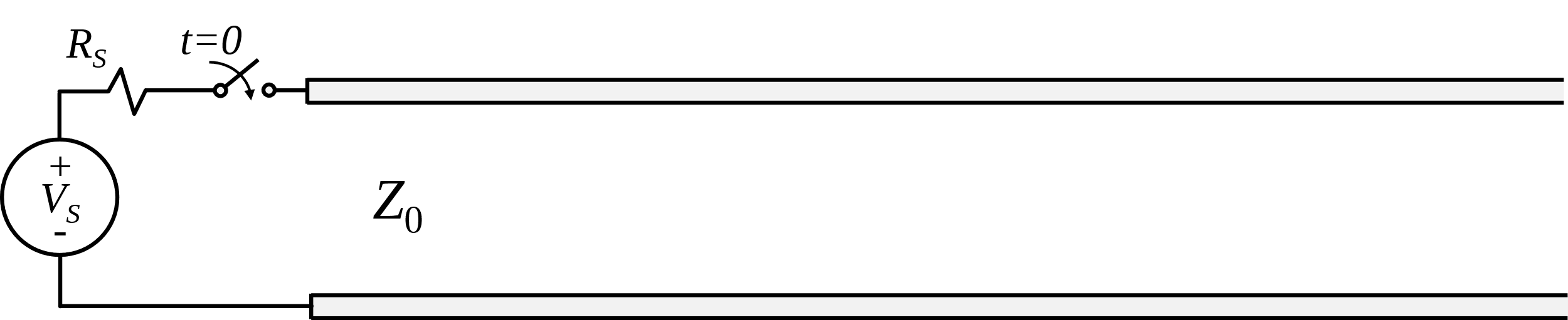
Figure 3. Semi-infinite transmission line.
The voltage wave progresses only as fast as the line current can carry charge to the wave front to produce the change in voltage. The current wave can only be supported on parts of the line where sufficient voltage exists to force the movement of charge. In other words, the voltage and current wave fronts must move along the line together.
A transmission line's characteristic impedance, Z0, is defined as the ratio of the voltage to the current in a forward-traveling wave. Suppose that at time t = t0 the wave front is located at z = z0, and at t = t0+Δt, the wave front is located at z = z0+Δz. During the time interval Δt, the total charge flowing out of the voltage source is I0Δt. During the same time interval, the voltage across the capacitance CΔz, associated with a short section Δz of the line, is raised from 0 to V0. This is accomplished by storing a charge equal to V0 C Δz on that section of the line. Thus,
From (11), the velocity of propagation, Δz/Δt, is , so the characteristic impedance is,
Example 1: Semi-infinite Transmission Line
Find an expression for the voltage and the current on the semi-infinite transmission line illustrated below.
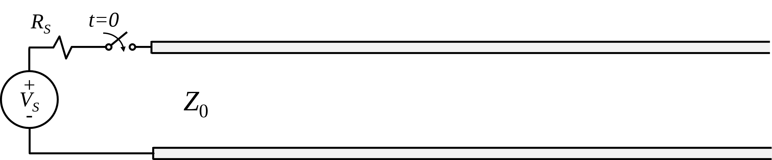
A DC source with open-circuit voltage Vs and source impedance RS is connected to the transmission line through a switch that closes at t = 0. At the moment the switch first closes, a voltage appears across the input to the transmission line, and current begins to flow. By Kirchhoff’s current law, the current into the transmission line, I0, equals the current delivered by the source. By Kirchhoff’s voltage law, and
In other words, the input to the transmission line looks like a resistor with impedance Z0 when the switch is first closed. Once current starts to flow on the transmission line, current and voltage wavefronts propagate down the line at velocity v. Since the line is infinitely long, these waves can propagate forever. The line draws a constant current from the voltage source. From the source's point of view, this transmission line behaves exactly like a resistor with a resistance equal to Z0.
In terms of the general solution to the wave equation (10), the arbitrary function must be equal to zero, since there is no mechanism to generate a wave going in the -z direction. At the input to the transmission line,
Therefore, F1(t) is equal to the unit step function U(t), and
The characteristic impedance has the same units as a resistance (ohms). The product of the voltage across and the current through a resistor represents power lost as heat. The product of the voltage across and the current through a real-valued characteristic impedance represents the power being carried away. It is lost to the source but not as heat. It takes the form of electromagnetic energy flowing down the transmission line.
Finite Length Transmission Lines
A finite-length transmission line behaves exactly like a semi-infinite transmission line during the first few moments after the excitation appears at the input. The transmission line’s termination cannot affect the signal at the input until the initial input has propagated down to the termination and back to the source.
Consider the transmission line with an open-circuit termination shown in Figure 4. As the switch is closed at t = 0, the voltage source supplies current to charge the line, and a wave is launched. Since this wave travels in the positive z direction, it will be referred to as a forward-traveling or incident wave. Until the wave reaches the termination at z = ℓ, this circuit behaves as if the transmission line were semi-infinite. However, when the incident wave reaches the open-circuit end of the transmission line, the current suddenly drops to zero. Back at the source end of the line, current continues to flow even after the incident wave reaches the termination, because it takes a finite time for the nature of the termination to be conveyed back to the source. In order to meet the boundary conditions at the termination, a new wave is launched. This is a backward-traveling or reflected wave. At all times, the sum of the incident and reflected waves must meet the boundary condition imposed by the termination. In this case, since the termination is an open circuit, the current in the reflected wave must be the negative of the current in the incident wave at z = ℓ. In other words,
where I+ (z,t) is the incident wave and I- (z,t) is the reflected wave.
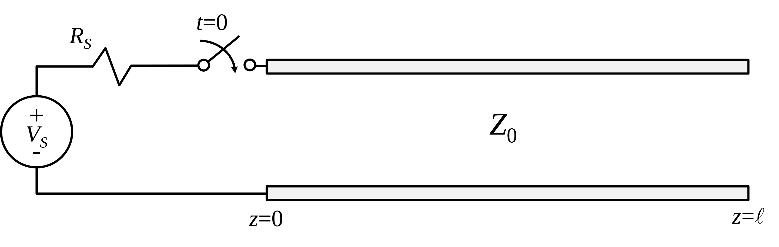
Figure 4. Finite length transmission line with open termination.
There is also a voltage associated with the reflected wave. The ratio of voltage to current in a reflected (-z directed) wave is equal to -Z0. The sign of Z0 indicates which direction the power is flowing relative to the arbitrarily defined direction of positive current flow. In this case, a positive Z0 represents power carried away from the source, while -Z0 represents power traveling back to the source. The current in the incident wave is I0 and the voltage is V0, the current in the reflected wave is -I0 and the reflected voltage is V0. At an open circuit termination, the current goes to zero and the voltage doubles.
Now consider the finite-length transmission line terminated in a resistance RL shown in Figure 5. When the incident wave reaches the termination, the voltage-to-current ratio is forced to equal RL. Unless RL = Z0, this requires a reflected wave.
Let’s let V + and I + represent the amplitude of the incident voltage and current waves, respectively. V - and I - will represent the amplitudes of the reflected voltage and current waves where,
When the incident wave reaches the point z = ℓ, the total voltage becomes V + + V - and the total current becomes I + + I -. By Ohm’s law, the ratio of the total voltage to the total current must be RL at z = ℓ. Therefore,
Combining Equations (18) and (19), we get
We can solve this equation to get the ratio of the reflected voltage to the incident voltage, which is also known as the voltage reflection coefficient,
This reflection coefficient is an important and useful concept in transmission line theory. Note that when Z0 = RL, Γ = 0. In other words, if a transmission line is terminated with a resistance equal to its characteristic impedance, there is no reflected wave. When the termination resistance is zero (short circuit), Γ = -1. When the termination resistance is infinite (open circuit), Γ = 1. The magnitude of the reflection coefficient is always less than or equal to 1.
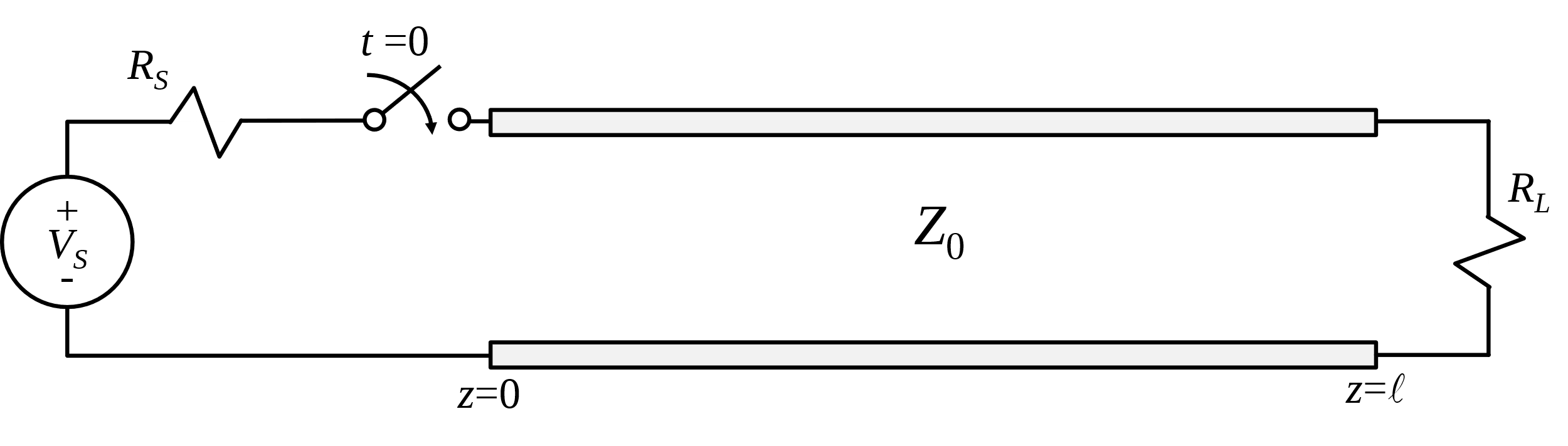
Figure 5. Terminated transmission line.
Example 2: Terminated Transmission Line
Plot the voltage and current distribution as a function of z for the transmission line shown below at times t = ℓ/4v, t = 3ℓ/4v, t = 5ℓ/4v, t = 7ℓ/4v, and t = 2ℓ/v.
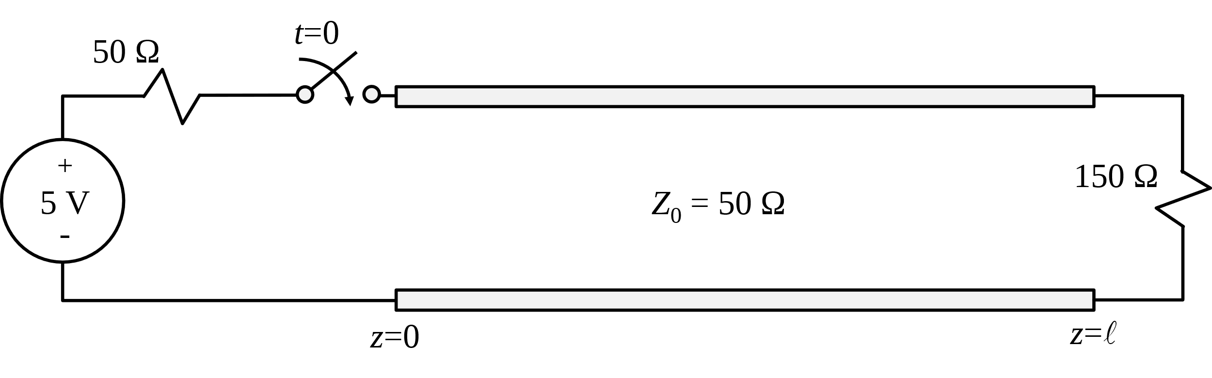
At t = 0+ (i.e., right after the switch is closed), the impedance presented to the source is the series combination of RS and Z0. Thus, the current drawn from the source is 5/(50+50) = 50 mA, and the voltage across the line at z = 0 is 2.5 volts. The incident voltage and current waves propagate down the line with velocity, v. At t = ℓ/4v, the wave front is at z = ℓ/4, as shown in the figure below.
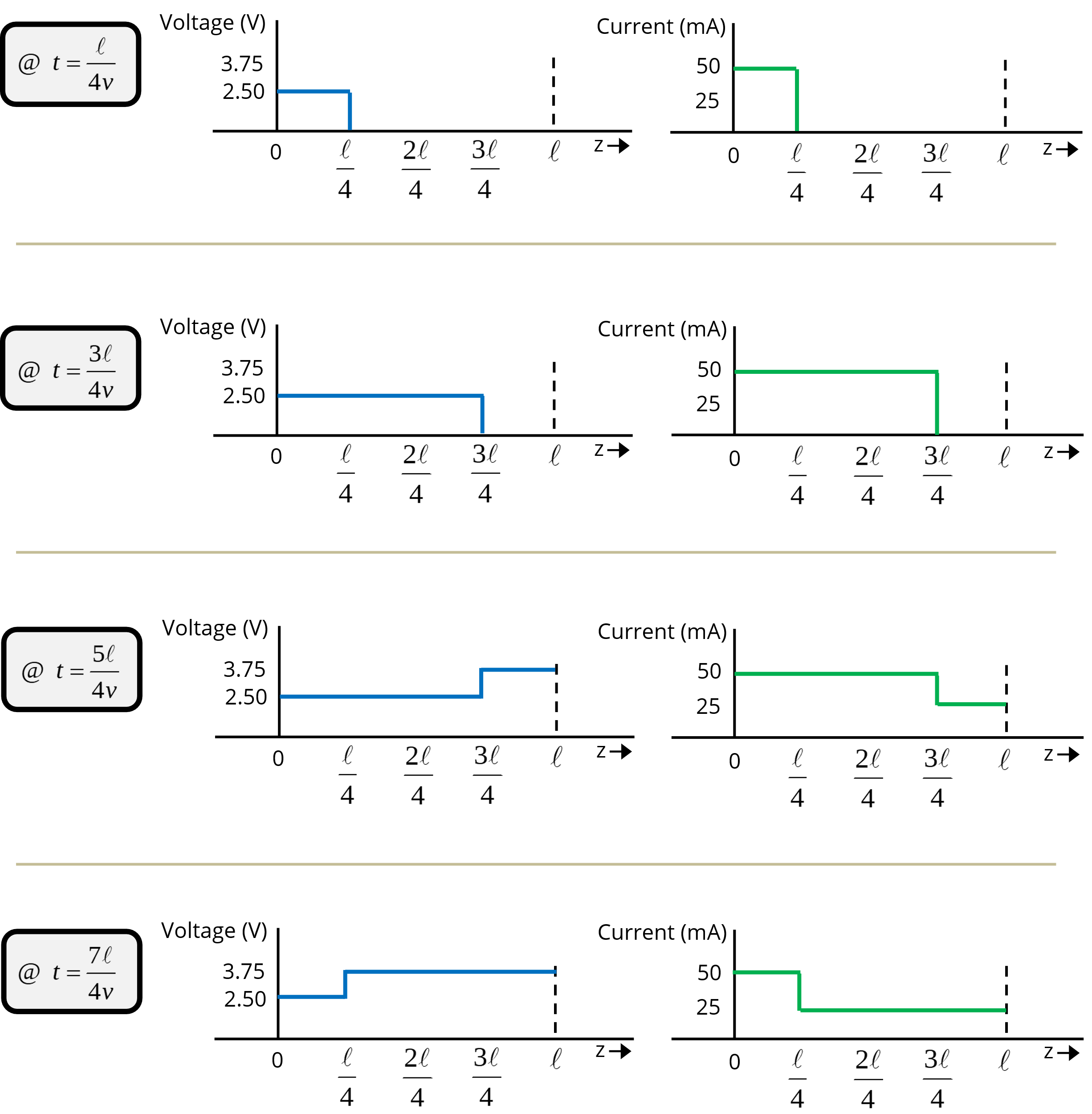

Note that up to this point, the load resistance has no effect. At t = 5ℓ/4v, the voltage and current waves have reflected off the termination. The voltage reflection coefficient, Γ, is (150-50)/(150+50) = ½. Therefore, the total voltage on the parts of the transmission line that have seen both the incident and reflected waves is 2.5 + 1.25 = 3.75 volts. The reflected current is -1/2 × 50 = -25 mA. Therefore, the total current on the parts of the line that have seen both the incident and reflected waves is 50 – 25 = 25 mA.
At t = 2ℓ/v, the reflected wave reaches the source. If the source impedance were not equal to the transmission line's characteristic impedance, another reflection would take place, and a second forward-traveling wave would be launched. In this example, however, the source impedance and characteristic impedance are equal. Γ = 0 at this end of the line, and there is no reflection. For t > 2ℓ/v, there is no change in the voltage and current on the line. The system has reached a steady-state solution.
Example 3: Transmission Line Voltage as a Function of Time
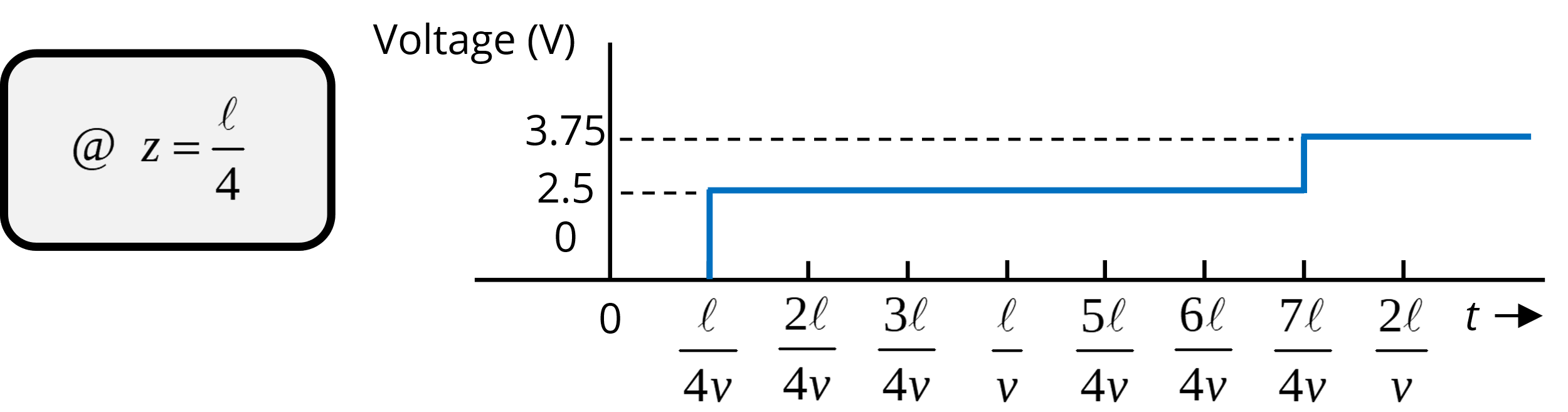
Plot the voltage as a function of time when measured at a position z = ℓ/4 along the transmission line in Example 2.
The figure below shows the voltage as a function of time as measured by a high-impedance oscilloscope located at a position z = ℓ/4. Note that even though the switch closes at time t = 0, nothing is observed until the incident wave passes by the oscilloscope position at time t = ℓ/4v. There is then no further change in the voltage until the reflected wave passes by at time t = 7ℓ/4v.
The Bounce Diagram
The voltage at any given position at any given time is the superposition of the voltages of every wave that has passed by that position up to that time. If both the source and the load impedance are not equal to the characteristic impedance, reflections occur at both ends of the line. In this situation, waves will bounce back and forth forever. However, since the reflection coefficient is always less than or equal to one, each reflected wave is smaller than the preceding waves, and the solution will converge to a steady state value. The steady state values are the voltages and currents that would have existed if the source had been directly connected to the termination with a pair of short wires.
Solving for the voltage and current waveforms on a transmission line that is mismatched at both ends can be complicated. A bounce diagram is a simple graphical way to track multiple reflections. A bounce diagram is a space-time diagram in which distance is plotted horizontally from the input to the load, and time is plotted vertically.
A bounce diagram for the transmission line in Examples 2 and 3 is shown in Figure 6. The locus of the wave front is represented by the end of a line that bounces back and forth, while moving down the face of the diagram. Since the wave front travels at constant speed, the angle of descent is constant, and the wave front traces a zigzag line as it bounces between the source and load. The amplitude of each wave front is written directly above each section of the line. The amplitude of a wave front is determined by multiplying the amplitude of the wave front above it by the reflection coefficient of the last termination it encountered.
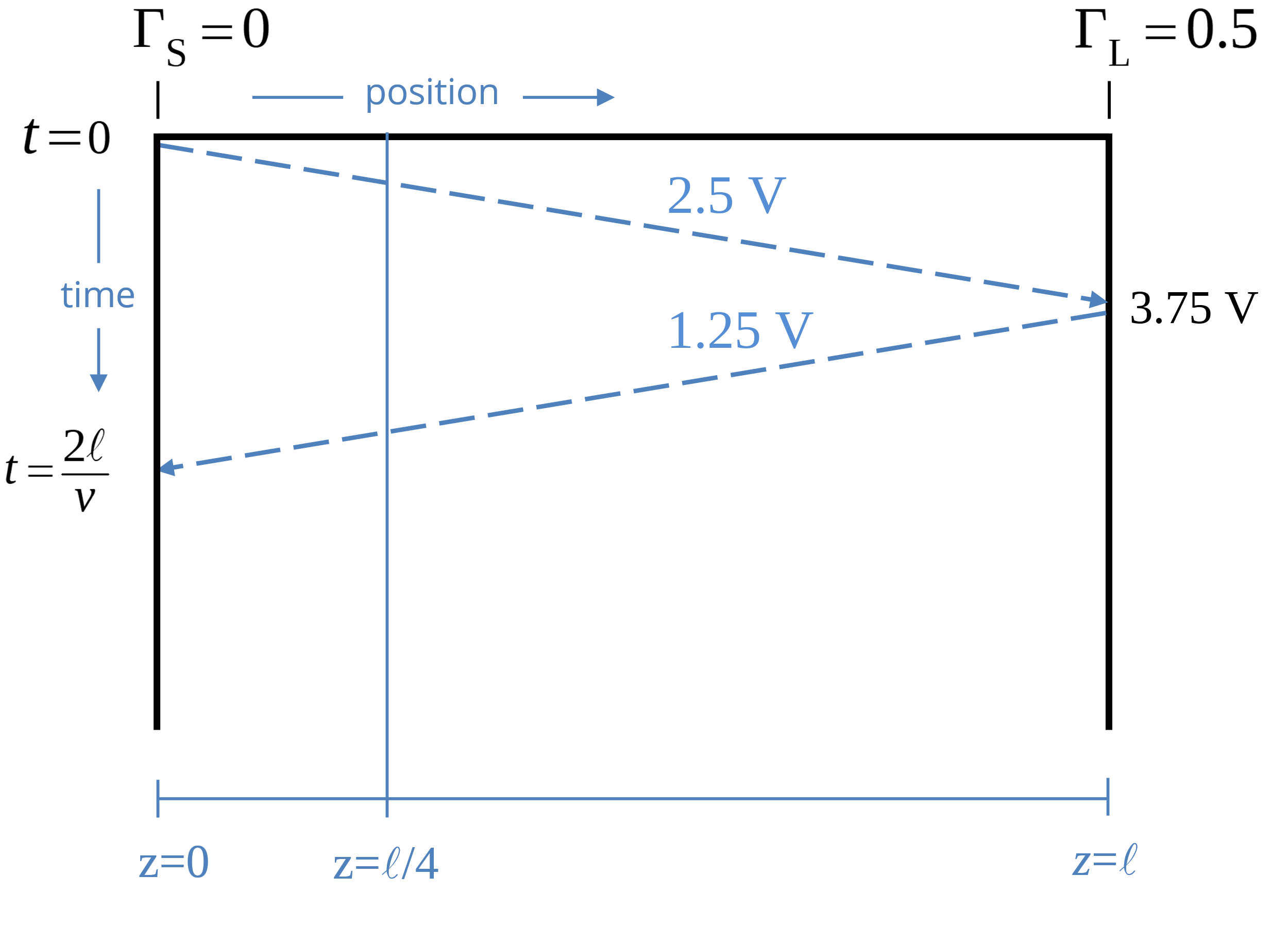
Figure 6. Bounce diagram for Examples 2 and 3.
Example 4: Voltage and Current as a Function of Time
The switch in the circuit shown in the figure below closes at t = 0. Plot the voltage and current as a function of time at z = ℓ/2.
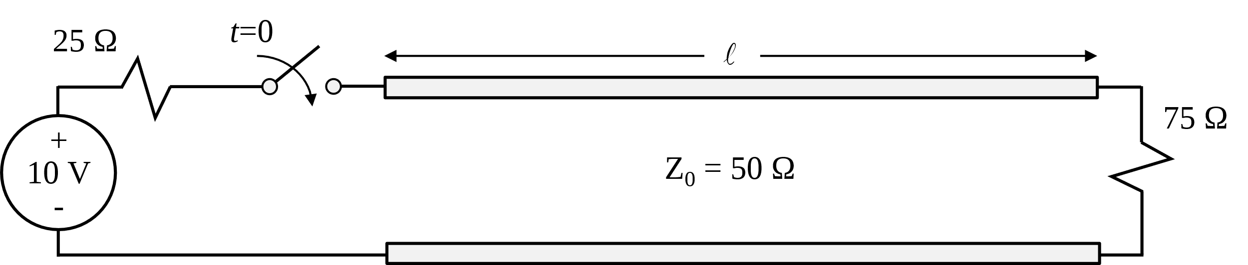
We will start by creating a bounce diagram for the voltage waveform. The voltage reflection coefficient at the source end of the line is The voltage reflection coefficient at the load end of the line is The bounce diagram corresponding to the voltage waveform is shown on the left in the figure below. The initial wave launched onto the line has a voltage determined by voltage division to be The voltage of the first reflected wave is The second reflected wave has amplitude The remaining wave amplitudes are found in a similar manner. Although the wave continues to bounce forever, note that the amplitudes become very small after several bounces.
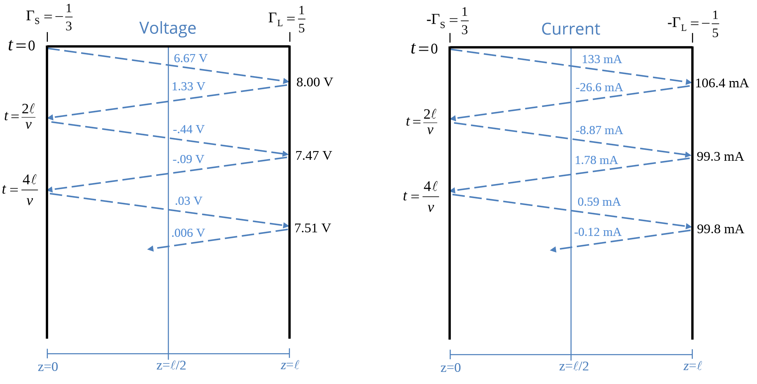
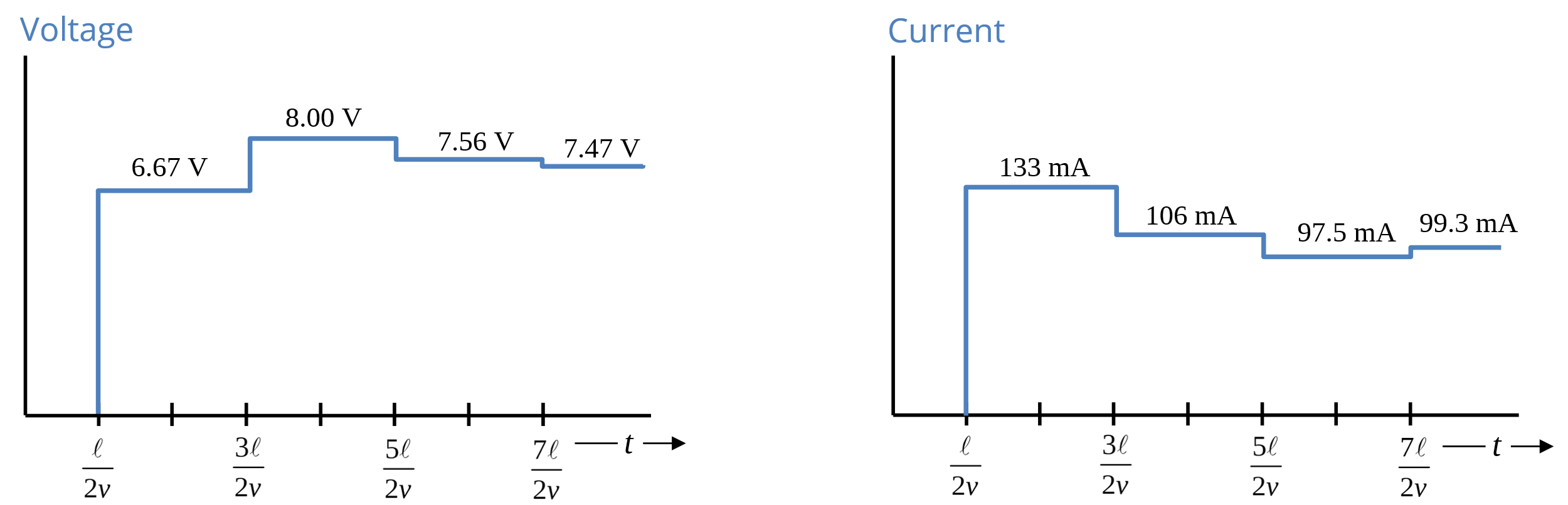
Once the bounce diagram has been completed, we can find the voltage at any position on the line as a function of time. The vertical blue line in the figure is a line of constant position at the center of the transmission line. The voltage is equal to the sum of the amplitudes of the wave fronts that have passed this position at any time. Therefore, until t = ℓ/2v, the voltage is zero since no wave fronts have crossed the dashed line. At t = ℓ/2v, the voltage jumps to 6.67 volts, the amplitude of the first wave front. At t = 3ℓ/2v, the voltage jumps to 8.0 volts, the sum of the first and second wave fronts. At t = 5ℓ/2v, the voltage decreases to 7.56 volts, the sum of the first three wave fronts.
A plot of the voltage at z = ℓ/2 as a function of time is shown on the left in the figure at the bottom of this example. As time progresses, the voltage converges to a constant value. This value is 7.5 volts, exactly the voltage that would have been dropped across the load if there were no transmission line. The voltage at all points along the line converges to this steady-state value.
We create a new bounce diagram to plot the current on the line. The bounce diagram for the current waveform is shown on the right in the previous figure. Note that the current reflection coefficient is equal to the negative of the voltage reflection coefficient. To avoid confusion, the symbol Γ refers to the voltage reflection coefficient. The current reflection coefficient is equal to -Γ.
The initial current waveform has an amplitude of 133 mA. The amplitudes of the reflected waveforms are determined using the same procedure used for the voltage waveforms. The figure below shows the current at z = ℓ/2 as a function of time. Note that the current converges to 100 mA, which is the value that would be delivered to the load if it were connected directly to the source.
Pulse Response of a Transmission Line Circuit
Figure 7(a) illustrates a transmission line circuit excited by a pulse with amplitude V0 and duration Δt. The pulse can be modeled as the superposition of two step functions. The first step function rises from 0 to V0 at time t = 0. The second step function falls from 0 to –V0 at time t = Δt. Viewed in this way, it is relatively straightforward to construct the bounce diagram in Figure 7(b). A plot of the voltage at the load end of the line is shown in Figure 7(c).
Quiz Question: How would the pulses in Figure 7(c) look if RS=Z0=50 Ω and the termination was a 5-pF capacitor?
If the source were matched to the transmission line, the initial pulse amplitude would be half the open-circuit source voltage. When the pulse arrived at the load end, the capacitor would initially look like a short circuit, and the voltage across the capacitor would be zero. However, the capacitor would charge with a time constant equal to Z0C. After 2.2 time constants (2.2 × 50 Ω × 5 pF = 550 ps), the capacitor would essentially become an open circuit with a reflection coefficient equal to 1.
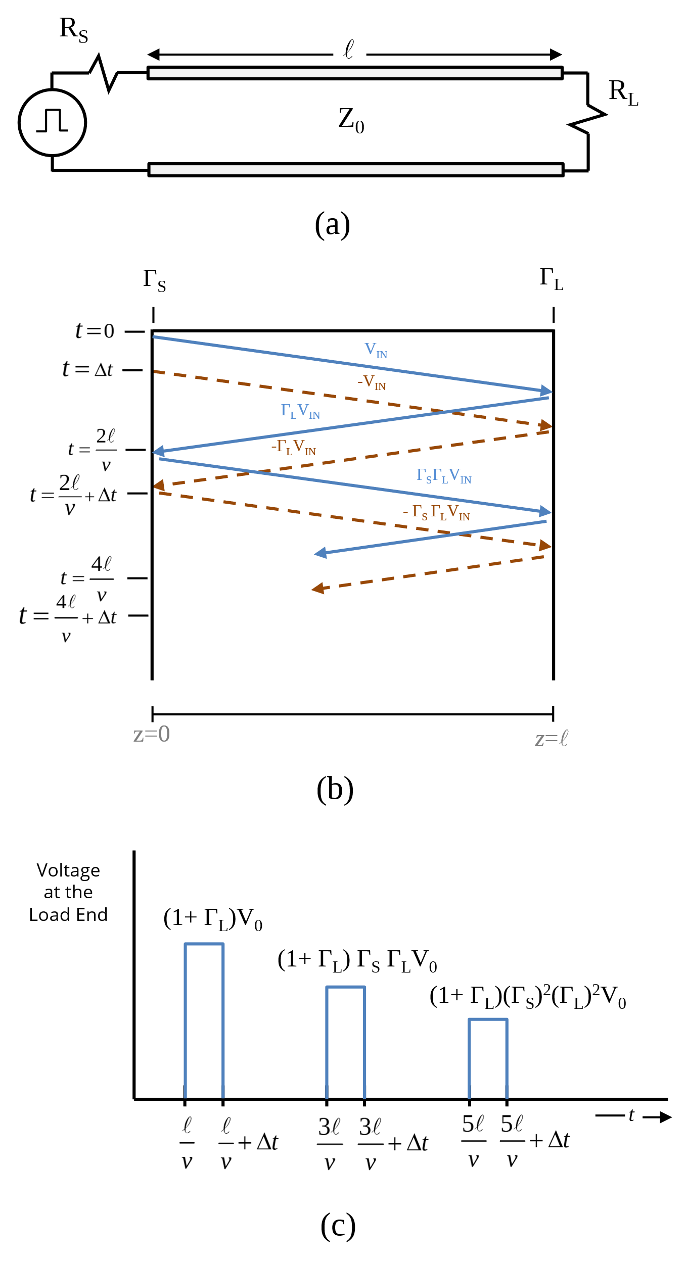
Figure 7. Pulse response of a transmission line circuit.
The voltage at the load would rise from 0 to the open-circuit voltage of the source in about 550 ps. When the falling edge of the pulse arrived at the load, the voltage would decay back to 0 with a fall time equal to its rise time. Because the source end is matched, no further reflected pulses would be observed. So, the pulse observed at the load end would be the same pulse that would have been observed if the load capacitance had been directly connected to the source (with a delay equal to the propagation delay of the transmission line).
Lossy Transmission Lines
So far, our analysis of the transmission line equations has assumed that the resistance and conductance per unit length are zero (i.e., R=G=0). Adding loss to the transmission line equations complicates their solution considerably. Pulses propagating along the line are both attenuated and distorted. If the loss is small, the distortion may be minimal, and the main effect of the loss may be a slight attenuation.
One method for analyzing lossy transmission lines is to represent them as lumped-element circuits (as in Figure 5.4) and use a SPICE circuit simulator. This method yields very accurate results if the length represented by each lumped-element section is less than about a tenth of a wavelength at the highest frequency of significance in the modeled waveform.
Another method is to represent the input signal in the frequency domain, calculate the transmission-line response, and reconstruct the time-domain signal. As the next section demonstrates, lossy transmission lines are easier to analyze in the frequency domain.