
Transmission Lines in the Frequency Domain
To analyze the response of a transmission line to a time-harmonic excitation, we must investigate solutions to the transmission line equations in the frequency domain. The lumped element model of a transmission line is shown in Figure 1. Phasor notation is used to represent the voltage V(z) and the current I(z) at a given frequency ω. The transmission line equations can now be written in phasor form,
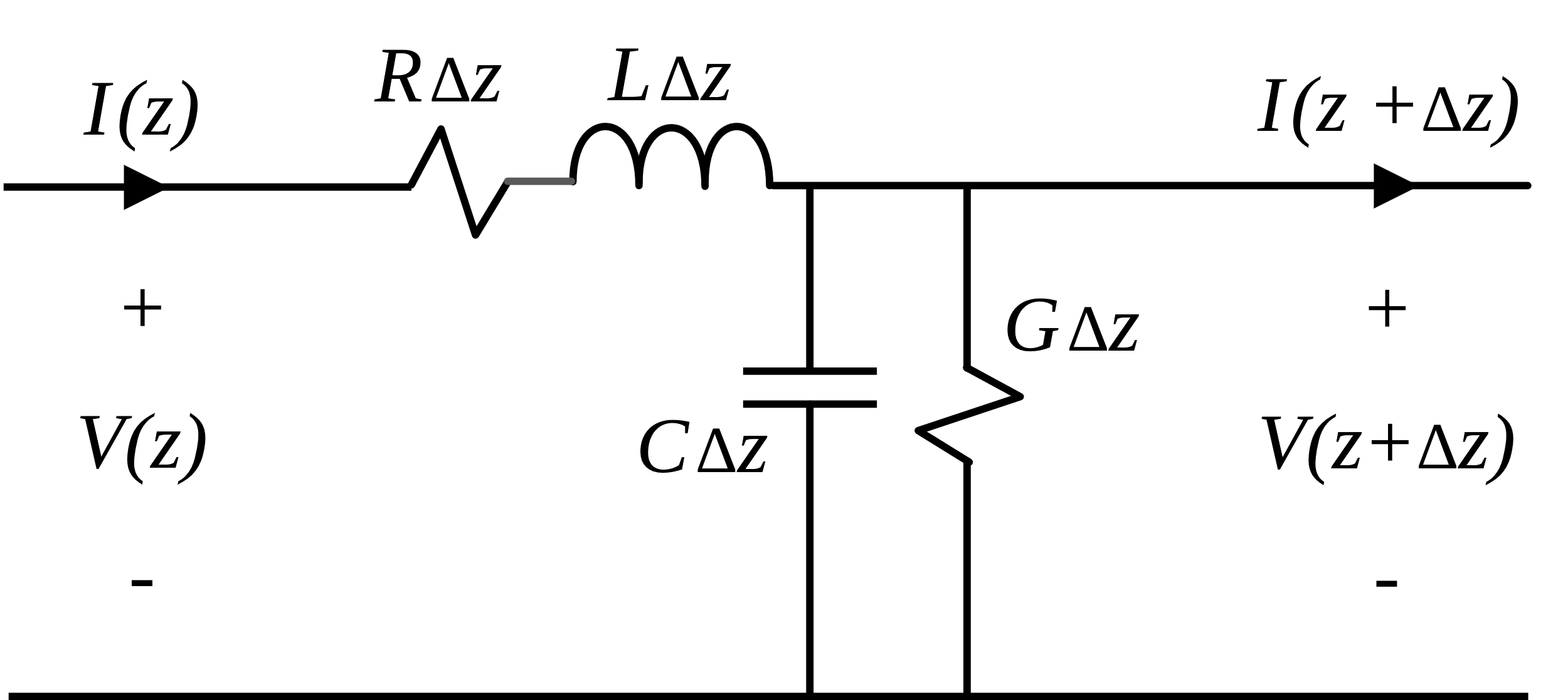
Figure 1. Lumped element model of transmission line section.
Taking the derivative of (1) with respect to z and combining it with (2) yields,
where,
Similarly, we can combine (1) and the derivative of (2) with respect to z to solve for the current,
In general, γ is a complex number whose value depends only on the properties of the transmission line,
where α is known as the attenuation constant, and β is the propagation constant of the line.
Equations (3) and (5) are ordinary differential equations with constant coefficients. They are wave equations with solutions of the form,
where V +, V -, I + and I - are complex constants whose values are determined by the boundary conditions.
We see from Equation (7) that the voltage V(z) at any point on the transmission line has two components V +e-γz and V -eγz. If we represent the complex value V + as its magnitude and phase, |V +| ejφ, and expand the first component to its full time-domain representation,
we see that it is of the form, F(t-z/v). This indicates that V + e-γz is a forward-traveling sinusoidal wave. Likewise, V - eγz is a backward-traveling sinusoidal wave. The voltage at any position is a superposition of these two sinusoids.
The term e-αz represents an exponential decay in the amplitude of the forward-traveling wave as it moves in the +z direction. The backward-traveling wave exhibits a similar, eαz, decay in the ‑z direction.
From (4) and (6), it is clear that the attenuation constant is,
Because this expression includes the square root of a complex number, there is no simple general expression for α in terms of R, L, G and C. However, for most transmission lines, the loss is relatively low at the frequencies of interest (i.e., R << ωL and G << ωC). In this case, we can use the low-loss approximation for α,
Typically, in cables and circuit board structures below 1 GHz, the conductor losses are greater than the dielectric losses, and the attenuation constant is approximately,
A wave traveling 1 meter along a transmission line is attenuated by a factor of eα. It is common to express the attenuation of a transmission line in dB/m,
For low-loss cables, the value obtained in (13) can be multiplied by 1000 to express the attenuation in dB/km.
The attenuation is a function of resistance, and the high-frequency resistance is a function of frequency (due to the skin effect). At frequencies where skin effect dominates, the resistance scales with the square root of the frequency. This means the attenuation expressed in dB/km scales with the square root of the frequency. So, a cable with an attenuation of 3 dB/km at 1 MHz would be expected to have an attenuation of about 30 dB/km at 100 MHz.
Substituting (7) and (8) into (1), we can show that,
Using (4), we get,
Since this must be true for all z,
Z0 gives the ratio of voltage to current in the forward-traveling component of the wave, or the negative of that ratio in the backward-traveling component. In general, however, the ratio of the total voltage to the total current on the line is a function of position.
Once again, for convenience, we will define z = 0 to be the location of the load. Thus, the load impedance, ZL, is equal to the ratio of the total voltage at z = 0 to the total current at z = 0,
Rearranging the terms in (18) yields,
As in the time-domain case, we define the voltage reflection coefficient to be the ratio of the reflected wave to the incident wave,
Comparing this result with the time-domain expression in the previous section, we see that ΓL is calculated from the load impedance and the characteristic impedance in the same way in both the time and frequency domains. In the frequency domain, however, the quantities Z0 and ZL are complex; therefore, ΓL may also be a complex quantity.
Lossless Transmission Lines in the Frequency Domain
Many practical transmission lines have relatively low loss and can be modeled as lossless (i.e., R ≈ G ≈ 0). Lossless lines have a real characteristic impedance,
and an imaginary propagation constant,
The voltage along a lossless line is given by,
The current along a lossless line is given by,
The impedance at z = -ℓ is found by combining Equations (23) and (24) with Equations (16) and (20),
Quiz Question:
At what length does the input impedance of a transmission line equal the load impedance?
From Equation (25), it is clear that Z(-ℓ) will equal ZL when the imaginary terms are zero. This occurs when tan βℓ = 0, or In other words, Z(‑ℓ) = ZL whenever the length of the transmission line is an integer multiple of a half wavelength.
Example 1: Shorted Lossless Transmission Line
Determine the voltage at all points along the shorted lossless transmission line in the figure below.
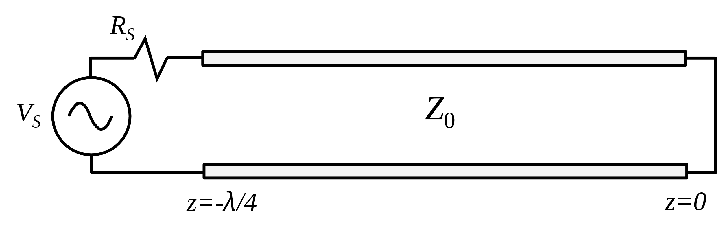
Note that we have defined z = 0 to be at the load end of the line for convenience in doing the calculations. Since the line is lossless, α = 0 and γ = jβ. The general solution for the voltage on the line (7) reduces to,
Applying the boundary condition at z = 0,
Therefore, and,
Applying Euler’s identity (e+jβz – e-jβz = 2j sin βz),
Now, we find the value of V+ by applying the other boundary condition,
Since , , and .
Substituting this value for V+ in the above equations, we get an expression for the voltage everywhere on the line,
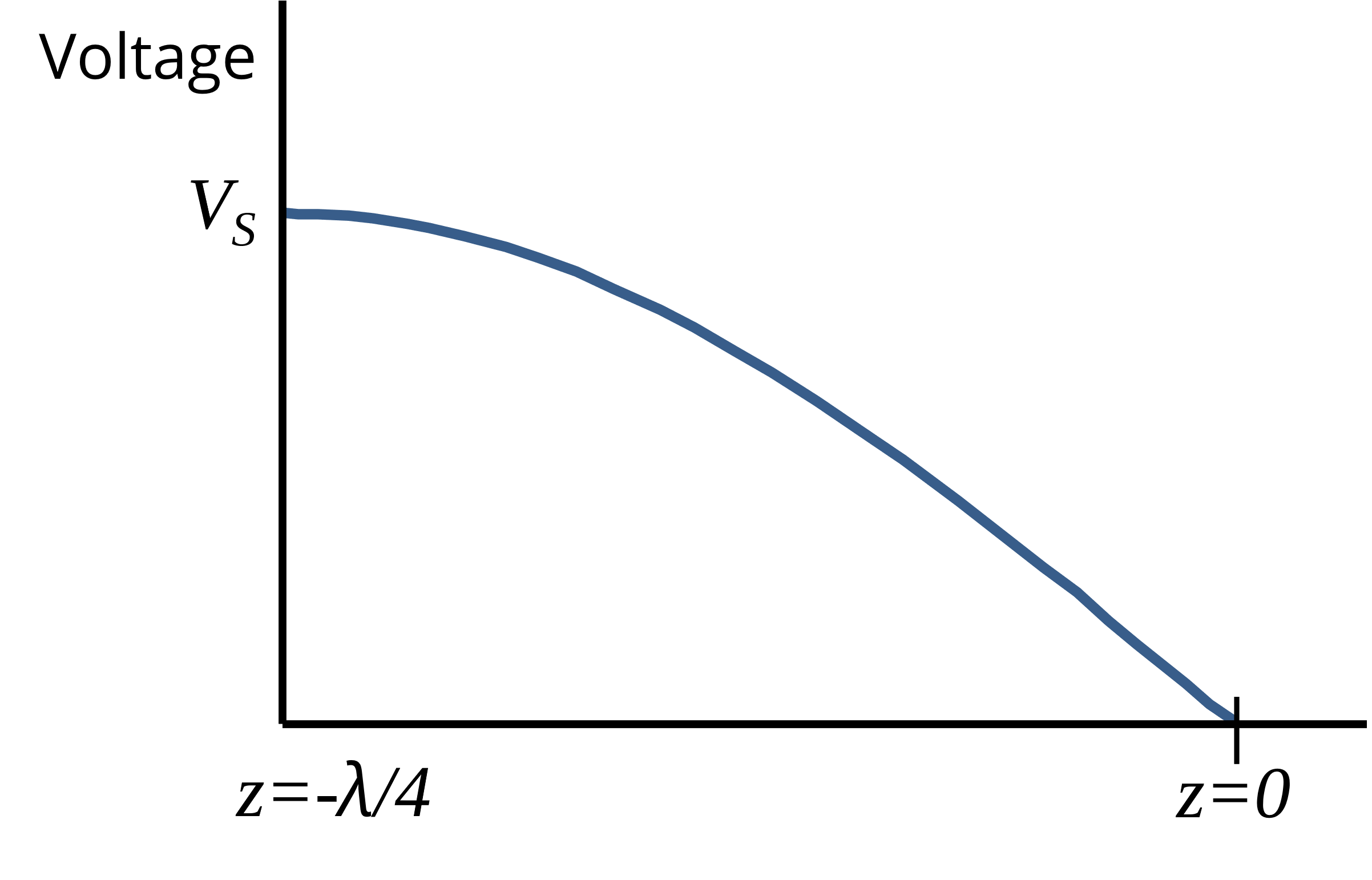
This sinusoidal voltage is plotted on the right. It is composed of two components: one forward-traveling and one backward-traveling wave. The load in this example is a short circuit and cannot dissipate power. Therefore, the time-average power moving in one direction must equal the time-average power moving in the other direction. The overall waveform V(z) does not propagate down the line. A waveform of this type is called a standing wave.
Example 2: Average Power Delivered to Load
Calculate the average power delivered to a 100-Ω load connected to a 5.0-volt, 25‑Ω source through a quarter-wavelength 50-Ω transmission line.
The configuration described in this example is illustrated below. There are a couple of approaches to solving this problem; however, the most straightforward is to find the input transmission-line impedance and calculate the average power delivered to it. Since the transmission line is lossless, all the power delivered is dissipated in the load impedance.

The impedance at the input to the transmission line is found using Equation (25),
Now the problem has been reduced to finding the power delivered to a 25‑Ω load from a 5.0-volt, 25-Ω source,