The Time-Domain Reflectometer

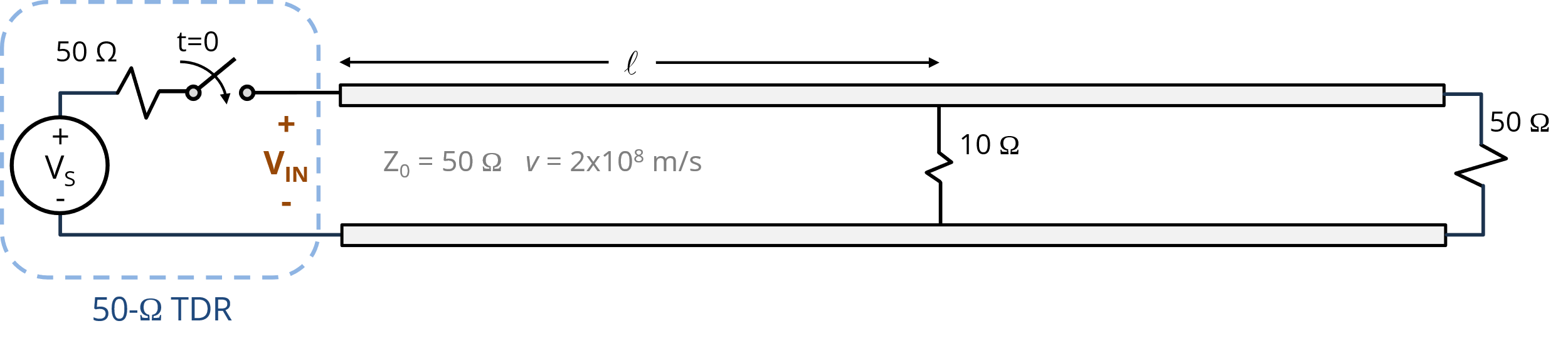
Figure 1. TDR connected to a transmission line with a 10-Ω shunt discontinuity.

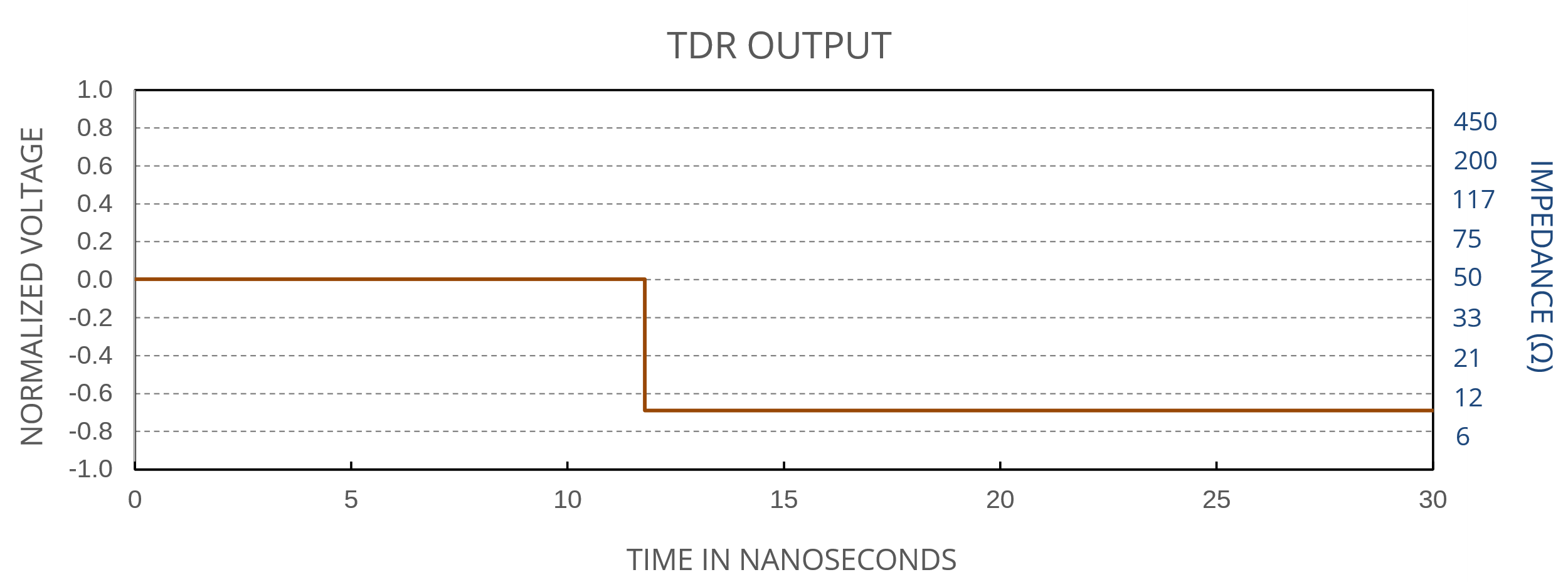
Figure 2. TDR output for a 10‑Ω shunt discontinuity.

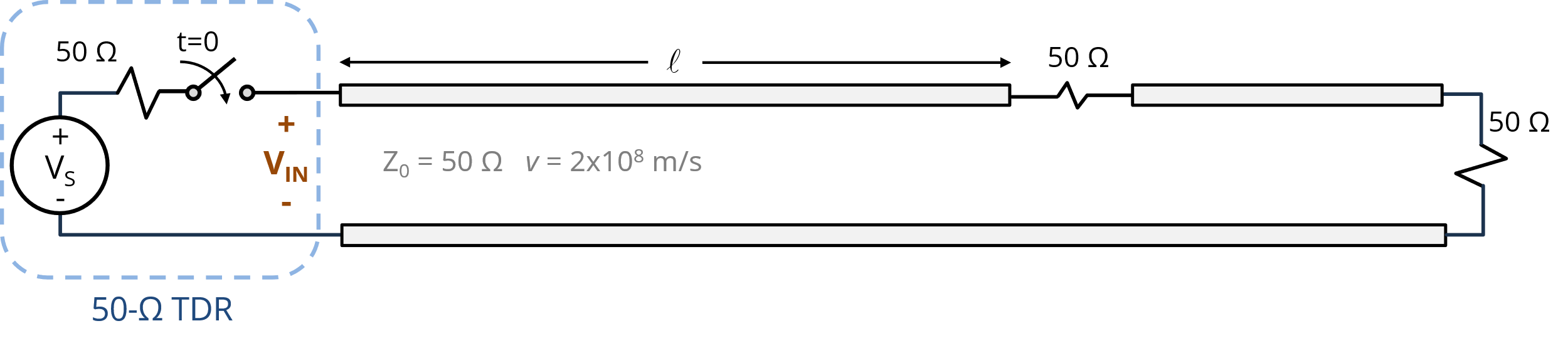
Figure 3. A series 50‑Ω discontinuity in a transmission line.

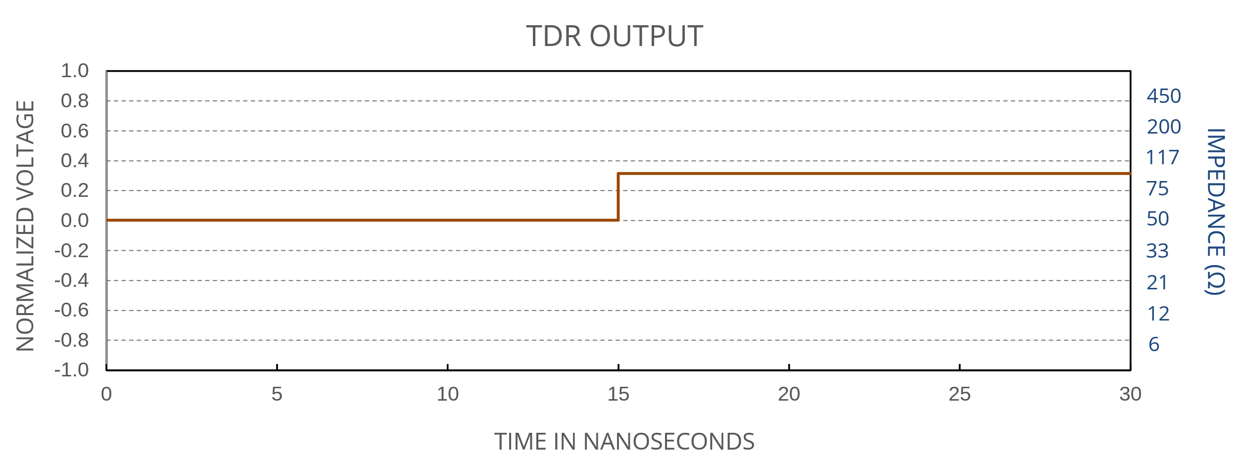
Figure 4. TDR output for a series 50-Ω discontinuity.

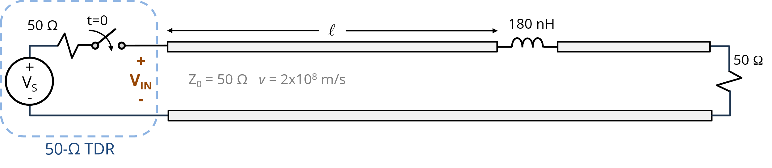
Figure 5. An inductive discontinuity in a matched transmission line.

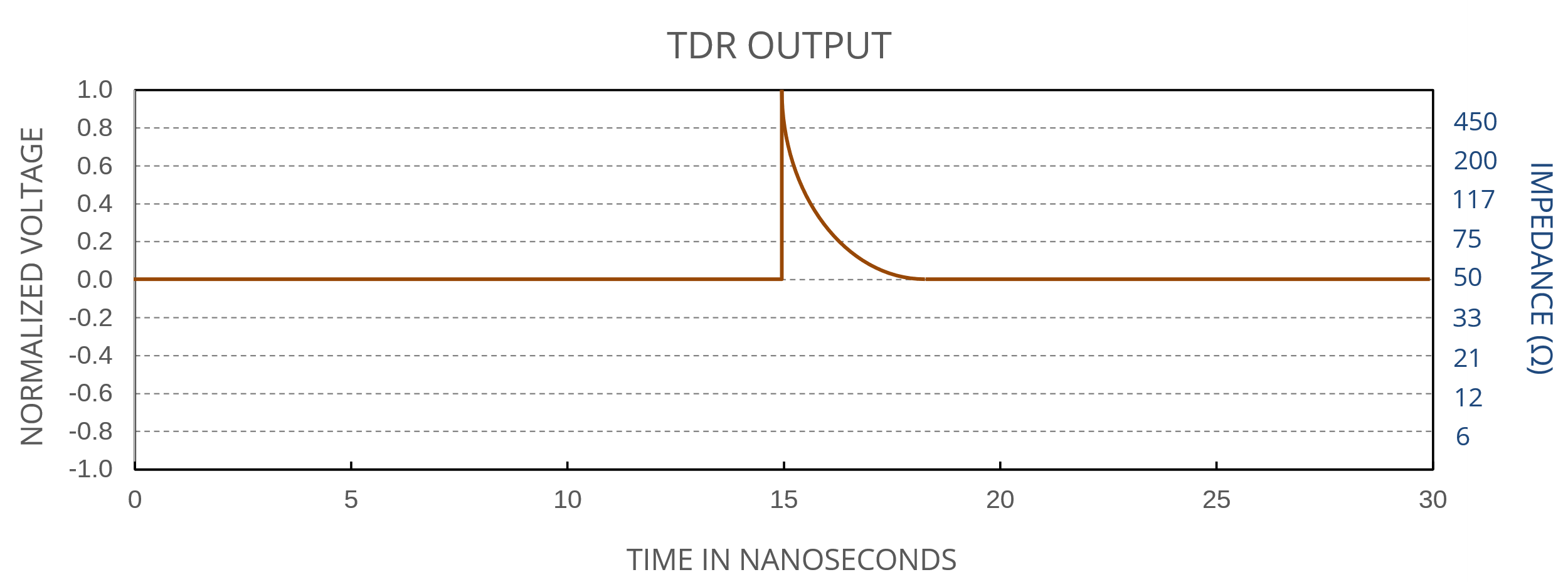
Figure 6. TDR output for a series inductance discontinuity.

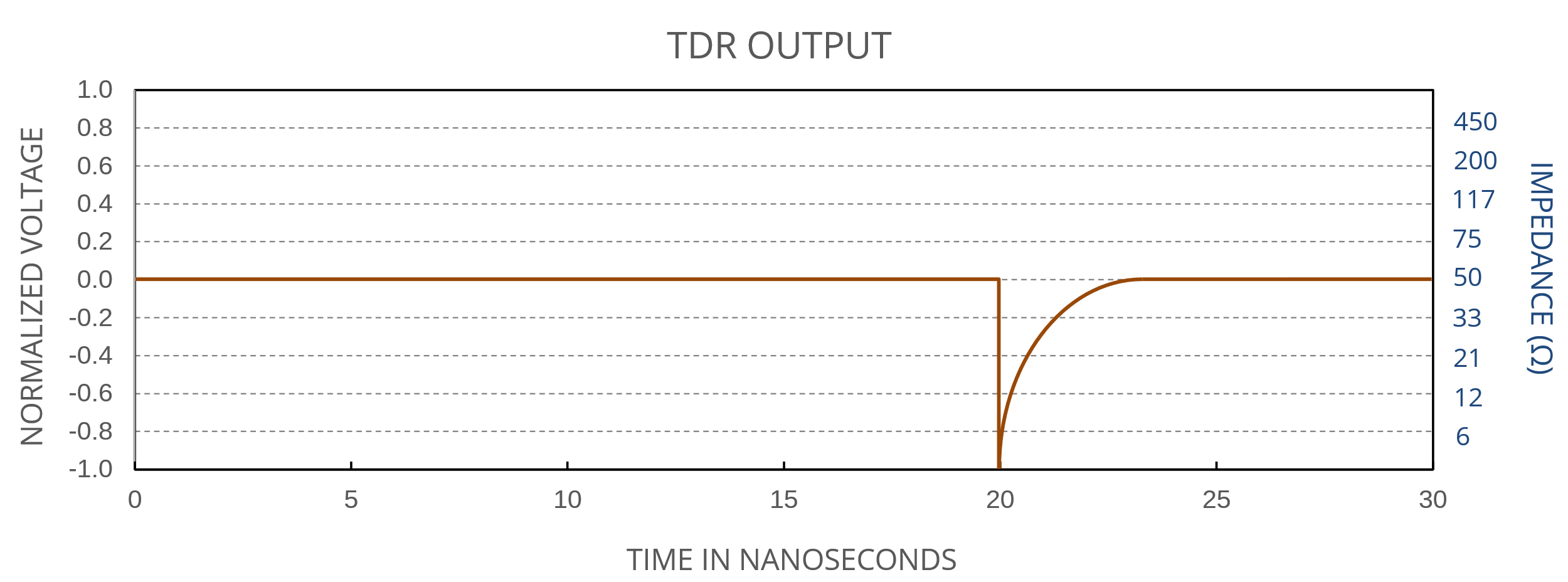
Figure 7. TDR output for a shunt capacitance discontinuity.

Ideally, a matched transmission line has a constant impedance from the signal source to the signal termination. In real systems, however, interconnections, parasitic coupling, and design tolerances contribute to impedance variations that can reflect some of the signal power back toward the source. The time-domain reflectometer (TDR) is a measurement instrument designed to locate and quantify unintended reflection sources.

A TDR works by applying a step change to the voltage across the input of a transmission line and monitoring the voltage at that point. If the line has no discontinuities and is perfectly matched, no change in the voltage at the input will be observed after the initial step. However, any discontinuity in the transmission line’s impedance will reflect some of the signal back to the source, where it can be recorded.

Figure 1 illustrates a TDR connected to a 50‑Ω transmission line with a 10‑Ω discontinuity located a distance l from the source end. The measurement of the input voltage begins with the switch closing at t=0 and is plotted in Figure 2. The vertical scale in this plot is offset by V_S/2 and normalized. The relative voltage plotted is,

$Normalized Voltage = \frac{V_{I N} - \frac{V_{S}}{2}}{\frac{V_{S}}{2}} = 2 (\frac{V_{I N}}{V_{S}}) - 1 .$

This unitless value is equal to the amplitude of the reflection coefficient. The plot in Figure 2 shows that the initial normalized voltage is zero, corresponding to a measured voltage of V_S/2. This is what we would expect from a 50‑Ω source that initially sees only the 50‑Ω characteristic impedance of the transmission line.

The voltage step propagates down the line until it reaches the 10‑Ω resistor. At that point, the wave sees the 10‑Ω resistance in parallel with the 50‑Ω impedance of the remaining transmission line. The parallel combination of these resistances is 8.33 Ω. The sudden change in impedance produces a reflected voltage step with an amplitude,

$V_{r e f l e c t e d} = Γ V_{i n c i d e n t} = \frac{Z_{L} - Z_{0}}{Z_{L} + Z_{0}} (\frac{V_{S}}{2}) = \frac{8.33 - 50}{8.33 + 50} (\frac{V_{S}}{2}) = - 0.766 (\frac{V_{S}}{2}) .$

After 12 ns, the reflected wave reaches the TDR, and the observed voltage takes on a new value,

$V_{I N} = V_{i n c i d e n t} + V_{r e f l e c t e d} = \frac{V_{S}}{2} - 0.766 (\frac{V_{S}}{2}) = 0.234 (\frac{V_{S}}{2}) .$

Using (5.54), this value of V_IN translates to a normalized value of -0.766, which is the reflection coefficient at the discontinuity.

If we know the reflection coefficient at the discontinuity, we can determine the impedance of the discontinuity using the equation,

$Z_{L} = Z_{0} \frac{1 + Γ}{1 - Γ} .$

In this way, we can map any reflection coefficient value in our 50‑Ω system to a resistance. This mapping is indicated by the vertical scale on the right side of the plot in Figure 2.

The plot in Figure 2 indicates not only the impedance at the discontinuity but also its location. Note that the voltage step occurs after 12 ns. This is the time it took for the wave to propagate from the TDR to the discontinuity and back. Since the velocity of propagation in the line is 2 x 10⁸ m/s (as indicated in Figure 5.17), the distance to the discontinuity is,

$ℓ = \frac{1}{2} (2 \times 10^{8} m/s) (12 \times 10^{- 9} s) = 1.2 m .$

Figure 3 shows another transmission line configuration with a 50‑Ω discontinuity in series with the conductors. The TDR output corresponding to this configuration is shown in Figure 4. The overall impedance at the discontinuity is 100 Ω, and the 15 ns round-trip propagation time indicates it is 1.5 m from the TDR.

TDRs can also detect and identify reactive elements, such as inductances and capacitances. Figure 5 shows a transmission line with an inductive discontinuity (e.g., from a mismatched connector). The corresponding TDR output is shown in Figure 6.

Note that at the instant the step reaches the inductance, it behaves like an open circuit with a reflection coefficient of +1. In the steady state, the inductance looks like a short circuit, so the impedance at the discontinuity is 50 Ω and the reflection coefficient is zero. Since the RL circuit forming the discontinuity is a first-order circuit, the transition from the initial voltage to the steady-state voltage is exponential with a transition time equal to,

$t_{r} = 2.2 \frac{L}{R} = 2.2 \frac{180 \times 10^{- 9} H}{50 Ω + 50 Ω} \approx 4 ns .$

Figure 7 shows the TDR output for another discontinuity. It initially looks like a short circuit with a reflection coefficient of -1. In the steady state, the discontinuity is gone, and the impedance is that of a matched termination. This is consistent with the behavior expected from a shunt capacitor.

In this case, the 20-ns round-trip delay indicates the capacitance is 2.0 meters from the TDR. The 4-ns transition time indicates that the capacitor value is,

$t_{r} = 2.2 R C \Rightarrow C = \frac{t_{r}}{2.2 R} = \frac{4 \times 10^{- 9} s}{2.2 (50 Ω ‖50 Ω)} \approx 73 pF .$