RLC Circuits in the Time Domain
All circuits have inductance and that inductance often plays an important role in EMC and signal integrity models. Being able to quickly evaluate simple RL circuits is an important skill for EMC and signal integrity engineers.
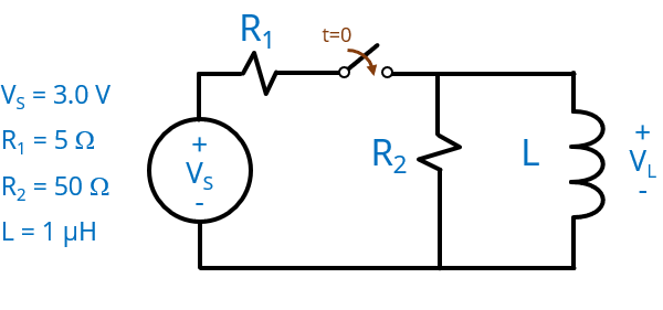
Consider the simple RL circuit shown in the figure. Suppose we want to model the voltage across R2 and the capacitor before and after the switch closes. If we start by writing node and mesh equations and solving differential equations, this relatively simple circuit will quickly become very difficult to solve. However, there's a basic set of steps than we can follow to quickly solve for all of the voltages and currents in any RC circuit that has only one capacitor. Those steps are listed below.
2. The current through an inductor is incapable of changing instantaneously. It can only change at a rate proportional to the voltage across it. At the moment immediately after the switch closes (t = 0+), the current through the inductor is equal to the current that was there before the switch closed. In that moment, it can be modeled as an ideal current source. In this example, the initial current was zero, so it can be modeled as an open circuit. The voltages and currents everywhere in the circuit at that moment can be found by opening the inductor and doing a DC analysis of the rest of the circuit. Note that while the current through the inductor can't change instantaneously, other circuit parameters can. In this case, the voltage across the inductor suddenly jumps from 0 to 2.73 V at t=0.
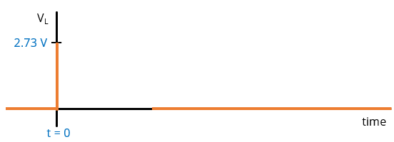
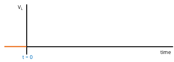
3. Eventually, the circuit will reach a steady state again. At that point, the inductor will behave like a short circuit again. So, we can determine the final steady-state voltages and currents by closing the switch and replacing the inductor with a short circuit. In this example, the steady-state voltage across the inductor is 0 volts. A plot of the voltage up to the closing of the switch and long after the switch closes is shown in the figure on the right.
4. All we are missing are the voltages and currents from the time immediately after the switch closes and the steady state. If the circuit has only one inductor, its behavior during that time is governed by a first-order differential equation. Solutions to that equation are exponentials. All of the voltages and currents in the circuit will transition from their initial state to their final state exponentially, starting at a rapid pace and slowing as they approach the steady state. These transitions are governed by the equations,
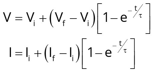
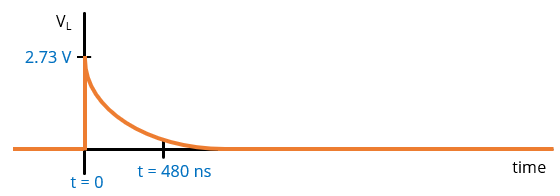
While these expressions look complicated, when plotted, they simply show a smooth exponential transition from the initial value to the final value. The exponential starts with a steep slope and ends with zero slope. The time constant associated with this transition is L/R, where R is the resistance viewed from the inductor terminals. In the case, the time constant is 220 nanoseconds. The 90-10% fall time is 2.2 time constants or about 480 ns. This transition is indicated in the figure on the right.
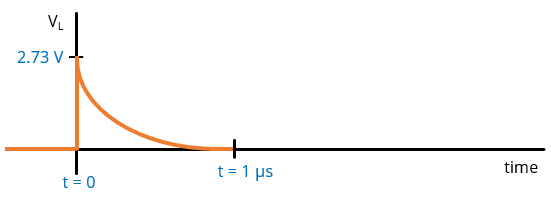
Now, let's use the same procedure to plot the voltage across the inductor assuming the switch opens again after being closed for 1 μs. At that point, the voltage has fallen to nearly 0 volts. The current in the inductor is the short-circuit current provided by the source, 3 V / 5 A = 0.6 A. The voltage up to the time the switch opens is plotted in the figure on the right.
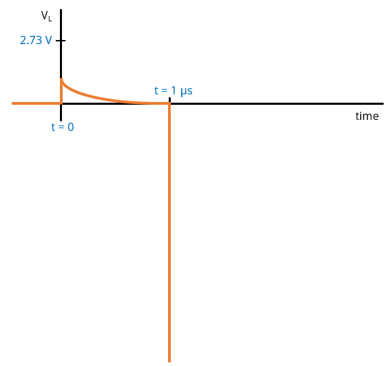
When the switch opens, the current through the inductor cannot instantaneously change. I briefly looks like a 0.6-A ideal current source. The switch is open, so all this current flows through the R2 resistor. This creates a voltage with a magnitude equal to 0.6 A x 50 Ω = 30 V. The current is flowing into the lower terminal of the resistor in the schematic, so the voltage amplitude is -30 V as indicated in the figure on the right.
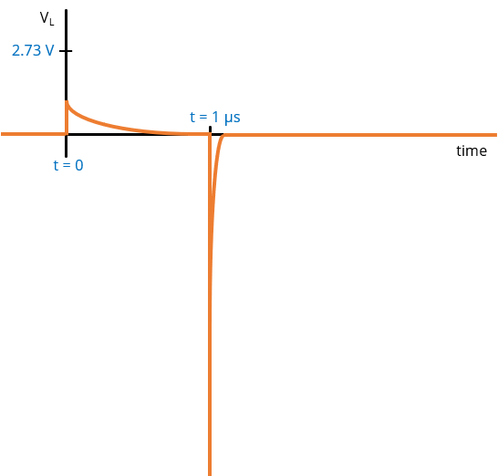
With the switch open, the energy will be drained from the inductor and the voltage across it will exponentially approach its steady-state value of zero. The time constant associated with this transition is L/R again, but this time the value of R is 50 Ω. The switch has disconnected the 5-Ω resistor and the source. The time constant is 1 μH / 50 Ω = 20 ns. The 10-90% transition time is 2.2 x 20 = 44 ns. The complete waveform is plotted on the right.