Resistance

In a circuit schematic, components are connected by lines. During a circuit simulation, those lines are assumed to be equipotential. No matter how much current they carry, the voltage on the line is the same everywhere.

In actual circuits, the lines on a schematic diagram are implemented using wires, traces on a circuit board, or metallization in a component. The circuit connections are made using materials such as gold, copper or aluminum. These materials are good conductors, but they are not perfect conductors. The finite conductivity of circuit connections ensures they will have non-zero resistance.

Most of the time, this resistance has a negligible impact on the circuit operation. However, there are situations where the resistance of circuit connections can be significant. When reviewing a circuit or system design, EMC engineers must be able to quickly estimate the resistance of various interconnects and determine whether this resistance is likely to be a factor in potential coupling or noise problems.

Fortunately, calculating the resistance of a circuit interconnect is not difficult, particularly if we only require order-of-magnitude accuracy. In circuit theory, Ohm’s law relates the voltage difference across a resistance to the current passing through it,

(1)

There is also a point form of Ohm’s law that is essential to electromagnetic field theory. In point form, Ohm’s law relates a current density to the electric field at a point,

(2)

where σ is the conductivity (in siemens/m) of the material in the region of the point.

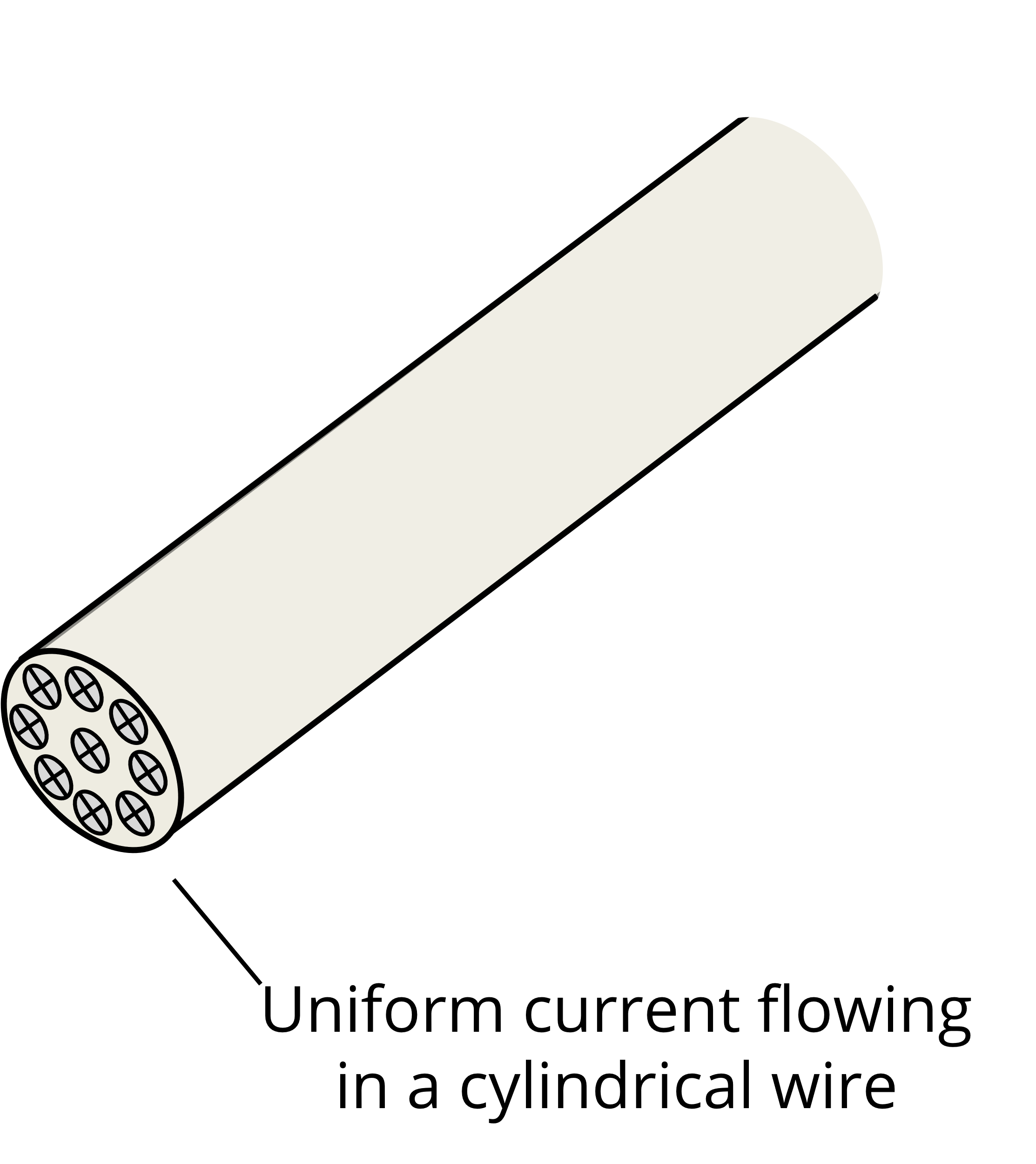
The resistance of a cylindrical object with a uniform current density, such as the wire illustrated in Figure 1, can be found by integrating the point form of Ohm’s law over a cross section,

(3)

The left-hand side of the above equation is the total current flowing through the cross-section. If the electric field strength is constant, then its magnitude can be expressed as the voltage from one end of the object to the other divided by the length, $\left|\overrightarrow{E}\right|=\raisebox{1ex}{$V$}\!\left/ \!\raisebox{-1ex}{$\text{ℓ}$}\right.$ , and Equation (3) can be written as,

(4)

Or, by rearranging the terms,

(5)

If the conductivity, σ, is a constant, then the resistance can be expressed as a function of the cross-sectional area, $A={\displaystyle {\int }_{S}ds}$ , as follows,

(6)

The derivation of Equation (6) assumes that the current is uniformly distributed throughout the cross section of the conductor. This is generally true for low-frequency currents (typically kHz frequencies and lower); however, electric fields (and therefore electric currents) have difficulty penetrating conductive materials at high frequencies. In the absence of other nearby conductors, the current density at high frequencies will peak at the surface and fall off exponentially inside the conductor, as illustrated in Figure 2. The rate at which the current density decays depends on the frequency of the current, the conductivity σ, and the permeability µ of the conductive material. In a good conductor (σ >>ωε), the current density inside a thick conductor is given by,

(7)

where J_s is the current density on the surface (at x=0) and x is the distance from the surface.

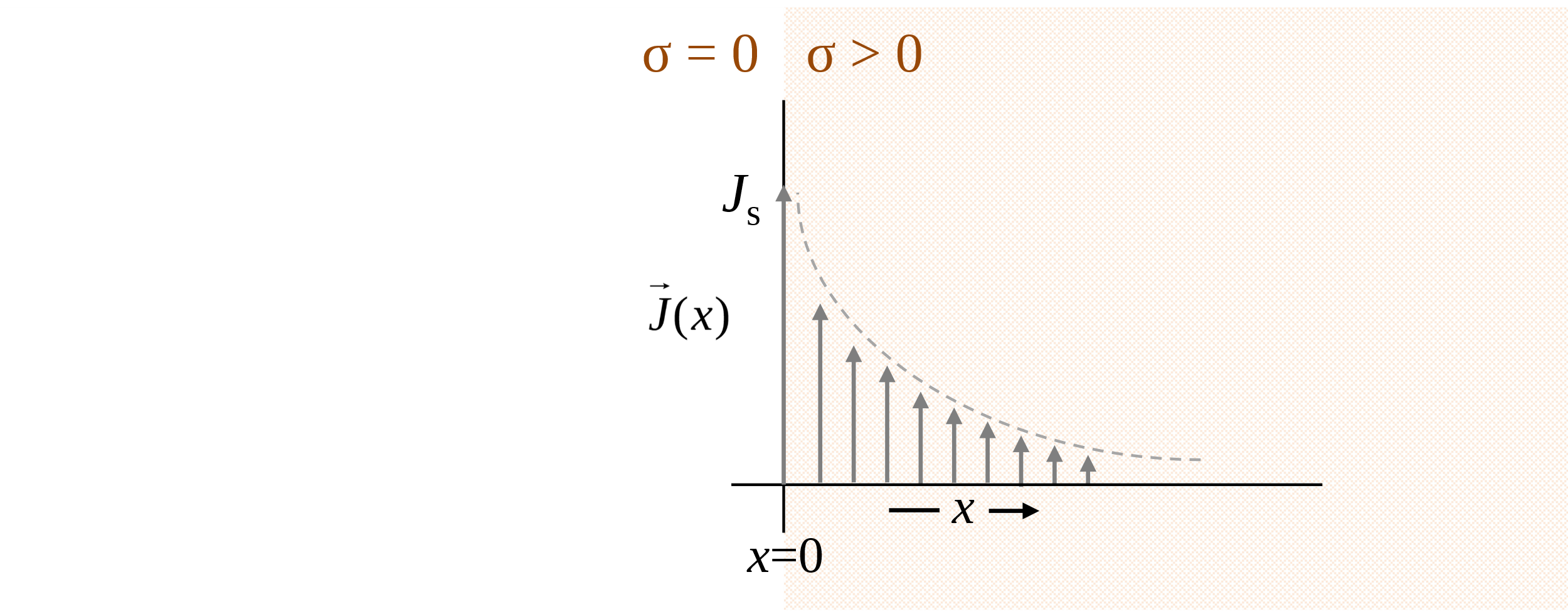
The distance at which the current density decays to 1/e of its value on the surface is called the skin depth, and is given by,

(8)

The total current flowing in a conductor that is many skin depths thick is approximately,

(9)

$I={\displaystyle {\int }_0^{\infty }{J}_S{e}^{-\raisebox{1ex}{$x$}\!\left/ \!\raisebox{-1ex}{$\delta $}\right.}dx=}{J}_S\delta \text{amperes}\text{.}$

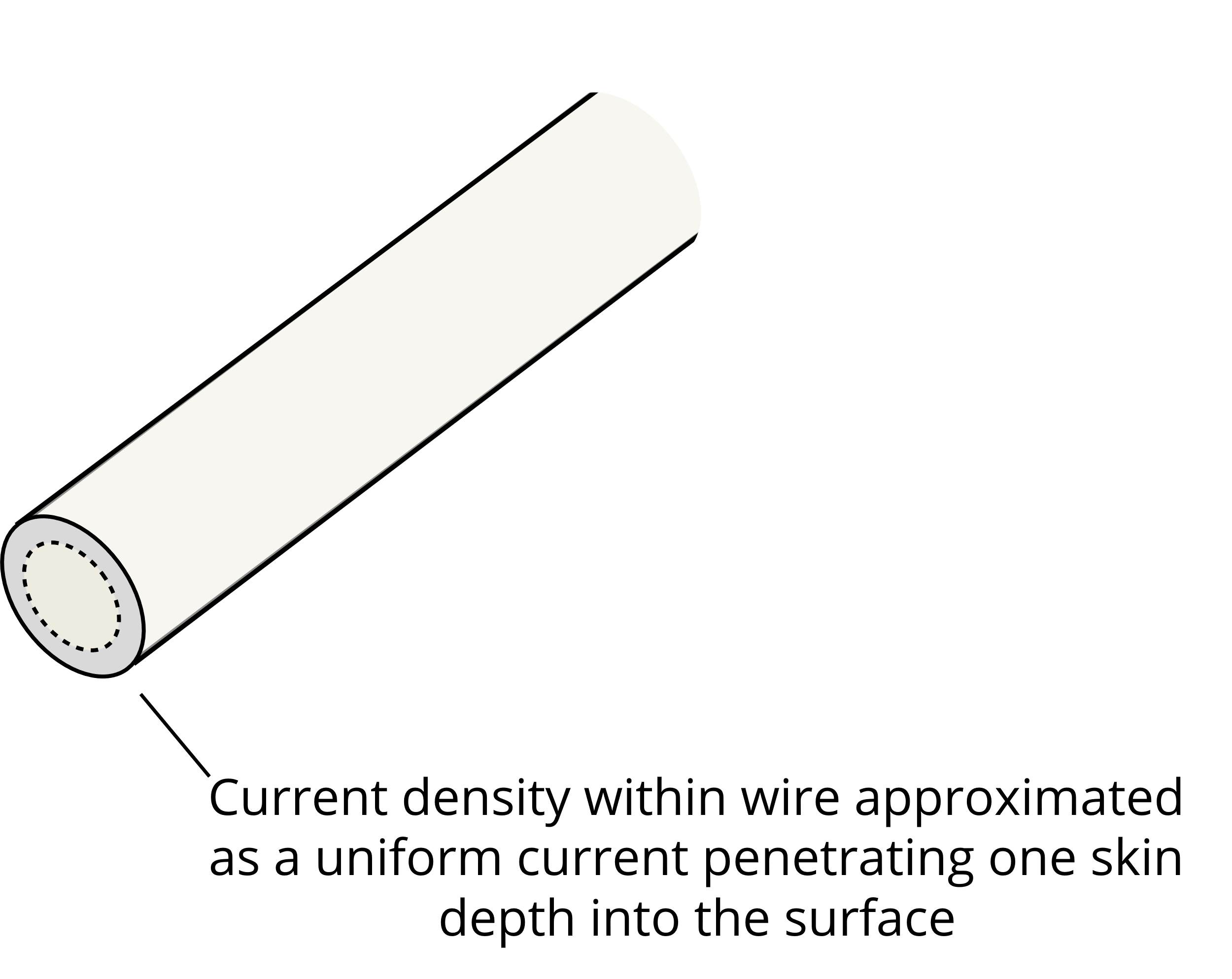
This is the same as the total current that would flow if the current were constant but only penetrated the surface a distance of one skin depth. When conductors are many skin depths thick, accurate and straightforward resistance calculations can be obtained by making this approximation. For example, to calculate the resistance of a round wire at high frequencies, we model the current distribution as having a constant amplitude within one skin depth of the surface and zero amplitude everywhere else, as illustrated in Figure 3. Using this approximation, a round wire of radius a has a total wire current of,

(10)

$J_S\left[\left(\pi a^2\right)-\pi {\left(a-\delta \right)}^2\right]\approx J_{S}2\pi a\delta \text{amperes}\text{.}$

The resistance of a round wire with length ℓ and radius a is then,

(11)

$R\approx \frac{\text{ℓ}}{\sigma 2\pi a\delta }\text{ohms}\text{.}$

Notice that Equation (11) is similar to the expression for the resistance at DC in Equation (6), except that the cross-sectional area of the wire, A, has been replaced by the equivalent current-carrying cross-sectional area, 2πaδ.

Example 2 illustrates how resistances are calculated at frequencies where the skin effect is not a factor and at frequencies where the skin effect is important. For the coaxial cable in this example, signals at 60 Hz see a resistance per unit length of 28 mΩ/m, while signals at 100 MHz see a much larger resistance per unit length of 923 mΩ/m. At frequencies where the skin depth is short relative to the conductor cross-sectional dimensions, the resistance per unit length of most signal conductors increases proportionally to the square root of the frequency.

Other factors, such as the proximity effect, can cause the current distribution in a conductor to be non-uniform. If the current distribution is known or can be approximated, Equation (3) can be used to find the conductor's resistance. If the current distribution is not known, numerical techniques can be employed. However, even when the precise current distribution is unknown, an estimate of the resistance based on the equations above is often sufficient.

Example 2: Resistance per Unit Length of a Coaxial Cable

Calculate the resistance per unit length of a coaxial cable at 60 Hz and 100 MHz. The conductors are copper with σ = 5.7 × 10⁷ S/m, µ = µ₀ = 4π × 10^-7 H/m. As indicated in the figure, r_a = 0.5 mm, r_b = 4.9 mm, and r_c = 5.0 mm.

At 60 Hz, the skin depth of the copper conductors is

${\delta }_{60Hz}=\frac{1}{\sqrt{\pi \left(60\right)\left(4\pi \times {10}^{-7}\right)\left(5.7\times {10}^7\right)}}=8.6\text{}\text{mm}\text{.}$

Since the thickness of the inner and outer conductors is much less than the calculated skin depth, the current density is uniformly distributed. The resistance per unit length of the cable is therefore,

$\begin{array}{c}{R}_{Inner-\text{}\text{}60\text{}Hz}=\frac{1}{\sigma A}=\frac{1}{\left(5.7\times {10}^7\right)\pi {\left(0.5\times {10}^{-3}\right)}^2}\\ =22.3\text{mΩ/m}\end{array}$

$R_{Outer-\text{}\text{}60\text{}Hz}=\frac{1}{\sigma A}=\frac{1}{\left(5.7\times {10}^7\right)2\pi \left(5\times {10}^{-3}\right)\left(0.1\times {10}^{-3}\right)}=5.6\text{mΩ/m}\text{.}$

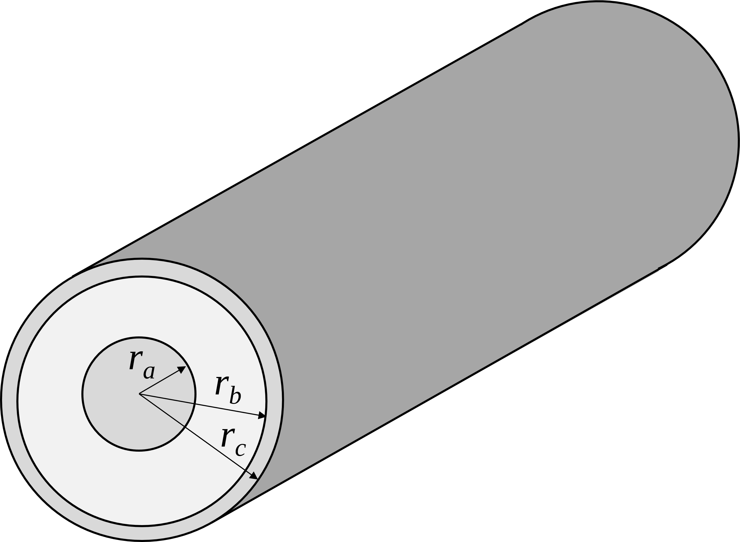
Since signal currents on a coaxial cable travel out on one of the conductors and return on the other, these two resistances are encountered in series. Thus, the total resistance per unit length at 60 Hz is the sum of the resistance of the inner and outer conductors,

$R_{60Hz}=22.3+5.6\simeq 28\text{mΩ/m}$

At 100 MHz, the skin depth of copper is

${\delta }_{100MHz}=\frac{1}{\sqrt{\pi \left({10}^8\right)\left(4\pi \times {10}^{-7}\right)\left(5.7\times {10}^7\right)}}=0.0067\text{}\text{}\text{mm}\text{.}$

Since the skin depth at 100 MHz is much less than the thickness of the conductors of the coaxial cable, we will use Equation (11) to calculate the resistance per unit length for the inner and outer conductors,

$\begin{array}{c}{R}_{Inner-\text{}100\text{}MHz}=\frac{1}{\sigma 2\pi a\delta }=\frac{1}{\left(5.7\times {10}^7\right)2\pi \left(0.5\times {10}^{-3}\right)\left(6.7\times {10}^{-6}\right)}=838\text{mΩ/m}\\ R_{Outer-\text{}\text{}100\text{}MHz}=\frac{1}{\sigma 2\pi a\delta }=\frac{1}{\left(5.7\times {10}^7\right)2\pi \left(4.9\times {10}^{-3}\right)\left(6.7\times {10}^{-6}\right)}=85\text{mΩ/m}\\ \\ R_{100MHz}=838+85=923\text{mΩ/m}\text{.}\end{array}$