
Modeling Discontinuities in Transmission Lines
Brief disruptions in a controlled-impedance signal path (e.g., due to electrical connections or layer transitions) can often be modeled as short transmission lines with a characteristic impedance different from the target impedance. When the disruptions are electrically short, they can usually be modeled using a single inductor or capacitor. This section discusses the appropriate value of the lumped elements used to model these disruptions.

Figure 1. Model of a discontinuity in a matched transmission line.

Figure 2. Simplified model of a discontinuity.
Consider the model for a discontinuity in a matched transmission line shown in Figure 1. Assuming the values of Z01 and Z02 are real numbers (i.e., the transmission lines are low loss), the termination of the transmission line segment on the left is simply the input impedance of the transmission line in the middle terminated by Z01, as shown in Figure 2.
The general expression for the input impedance of the transmission line representing the discontinuity is,
where β is the propagation constant of the transmission line (β = 2π/λ). If the length of the discontinuity ℓ is small relative to the signal wavelength, then βℓ is a small number and tan βℓ is approximately equal to βℓ. In this case, (1) reduces to,
Solving for the real and imaginary parts of Zin,
Since βℓ is small (i.e., βℓ<< 1), (3) reduces to,
Now, consider two cases: Z02 ≥ Z01 and Z02 ≤ Z01. If Z02 ≥ Z01 (i.e., the characteristic impedance of the discontinuity is greater than or equal to the characteristic impedance of the transmission line), then (4) can be written as,
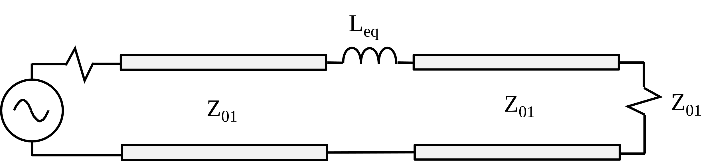
Figure 3. Simplified model of short discontinuity when Z02>Z01.
where Lℓ is the inductance per unit length of the discontinuity times the length. In other words, when the discontinuity has a characteristic impedance greater than the transmission line impedance, it can be modeled as a lumped inductor, as illustrated in Figure 3. The value of the equivalent inductance is,
For discontinuity impedances much larger than the transmission line impedance, the lumped inductance is approximately equal to the inductance per unit length times the length of the discontinuity. As the discontinuity impedance approaches the value of the transmission line impedance, the equivalent inductance decreases. The equivalent inductance is zero when the discontinuity has the same impedance as the transmission line.
Now let’s consider the case where an electrically short discontinuity has a lower characteristic impedance than the transmission line, Z02 ≤ Z01. In this case, it’s more convenient to solve for the input admittance (i.e., the inverse of the input impedance),
Applying the constraints, Z02 ≤ Z01 and βℓ<< 1, we get,
In other words, the real part of the input admittance is the same as the admittance of the termination. And the imaginary part of the input admittance is the same as the admittance of a capacitor with a value,

Figure 4. Simplified model of short discontinuity when Z02 < Z01.
Therefore, for Z02 ≤ Z01, we can model the discontinuity as a lumped capacitance, as shown in Figure 4.
Note that the equivalent circuits in Figures 3 and 4 apply to any short transmission line segment terminated with a resistance, not just discontinuities in a longer transmission line. A short transmission line segment terminated in a resistance lower than its characteristic impedance can be modeled as a lumped inductor in series with the termination resistor. A short transmission line segment terminated in a resistance higher than its characteristic impedance can be modeled as a lumped capacitor in parallel with the termination resistor.
If the termination resistance is much lower than the characteristic impedance, the lumped inductor's value is the transmission line's total inductance. If the termination resistance is much higher than the characteristic impedance, the value of the lumped capacitor is the total capacitance of the transmission line. If the termination impedance equals the characteristic impedance, the input impedance of the transmission line segment is equal to the termination resistance with no added inductance or capacitance.