Chapter 4 Lab Exercise: Harmonics of a Trapezoidal Waveform

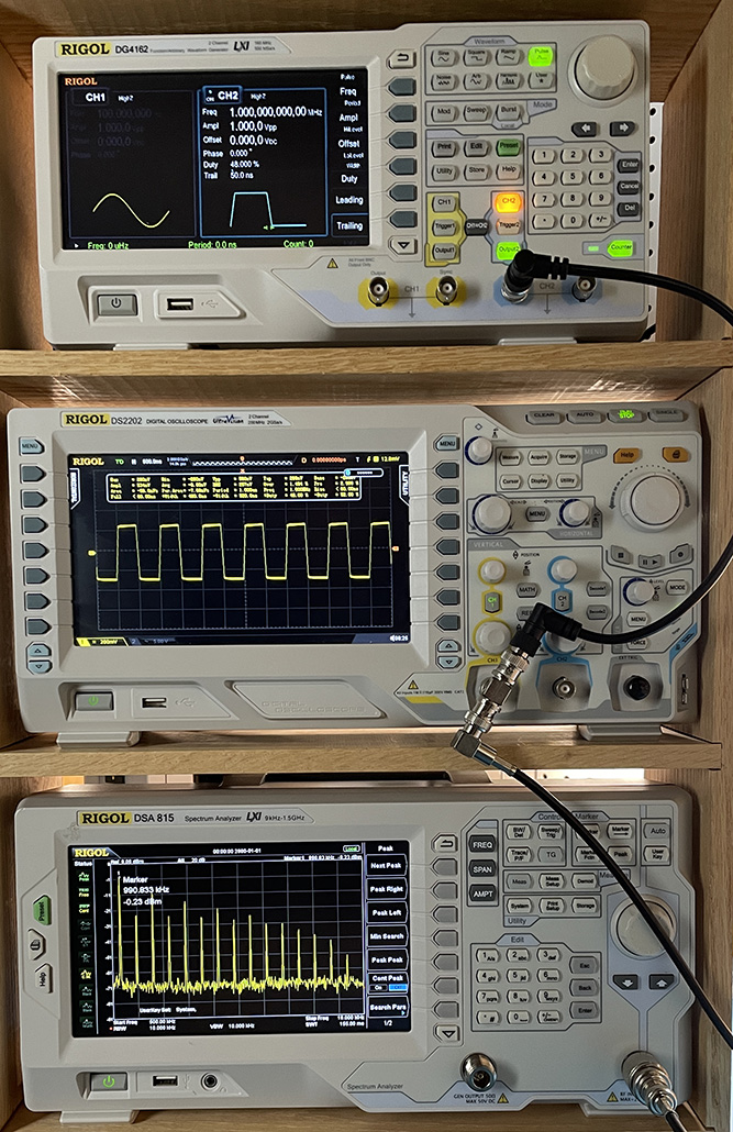
Many of the signals responsible for conducted and radiated emissions have waveforms that are essentially trapezoidal. For example, digital clock signals, binary data signals, and PWM control signals all have waveforms that switch between two voltage levels with relatively consistent rise and fall times. It is important for EMC engineers to understand how the various parameters of these waveforms in the time domain affect these signals in the frequency domain.   

Preparation:  Students should read Chapter 4 before starting this exercise. They should be familiar with the basic operation of traditional EMI test receivers. You may want to provide them with the transition times that they will measure, so that they can calculate the harmonic amplitudes before they come into the lab. 

Equipment Required:

• waveform generator
• oscilloscope with a bandwidth ≥ 500 MHz
• spectrum analyzer or EMI test receiver

Procedure:

Step 1: Connect the waveform generator to both the oscilloscope and the spectrum analyzer using coaxial cables and a T-connector. Use the 50-Ω input for the oscilloscope.

Step 2: Set the spectrum analyzer to view frequencies from 500 kHz to 50 MHz. Set the resolution bandwidth to 10 kHz.

Step 3: Set the waveform generator to produce a 500 ns pulse with a 1000 ns repetition rate and a peak-to-peak amplitude of 1 volt as displayed on the oscilloscope. Ensure that the waveform generator is set to switch as fast as it is capable. Note the rise-time and fall-time of the displayed waveform. 

Step 4: Put a marker on the harmonic appearing at or near 1 MHz on the spectrum analyzer display. Using the formula in Chapter 4, the amplitude of the first harmonics should be 0.45 times the peak-to-peak voltage. This would be 1-volt peak is 0.45 V_rms, which is 93 dB(μV) or 6 dBm. Calculate the difference between the calculated amplitude and the measured amplitude for each of the odd harmonics from 1 to 15. 

Step 5: Change the rise-time and fall-time of the pulsed waveform to 40 ns. If the waveform generator doesn't allow the transition time to be adjusted, this can be accomplished by placing a capacitor in parallel with the signal path. The value of the capacitor required will depend on the generator output impedance but will be on the order of 2 nF. 

Step 6: Observe the waveform in the time domain. Does it still resemble a digital clock signal? Note the amplitude of the first 15 harmonics and compare the measured values to the expected values. By how much was the harmonic at 15 MHz reduced? 

Step 7: Observe the effect that the change in transition times has on the harmonics from 30-50 MHz. Are they also attenuated? If not, then why not? (Note that the answer to this question will depend on the method used to slow the transition time.) 

Step 8: Decrease pulse width to 480 ns. Repeat the measurement with fast and slow transition times. Are there any significant differences?

Step 9: Decrease pulse width to 100 ns. Repeat the measurement with fast and slow transition times. Are there any significant differences? What effect does the change in transition time have on the pulse waveform in the time domain? 

Notes: 

Depending on the characteristics of the waveform generator and analyzer, a fundamental frequency other than 1 MHz can be chosen for this exercise.  

This lab exercise can also be performed using a digital oscilloscope with an FFT function.