
Chapter 4 Lab Exercise: Time and Frequency Domain Measurements
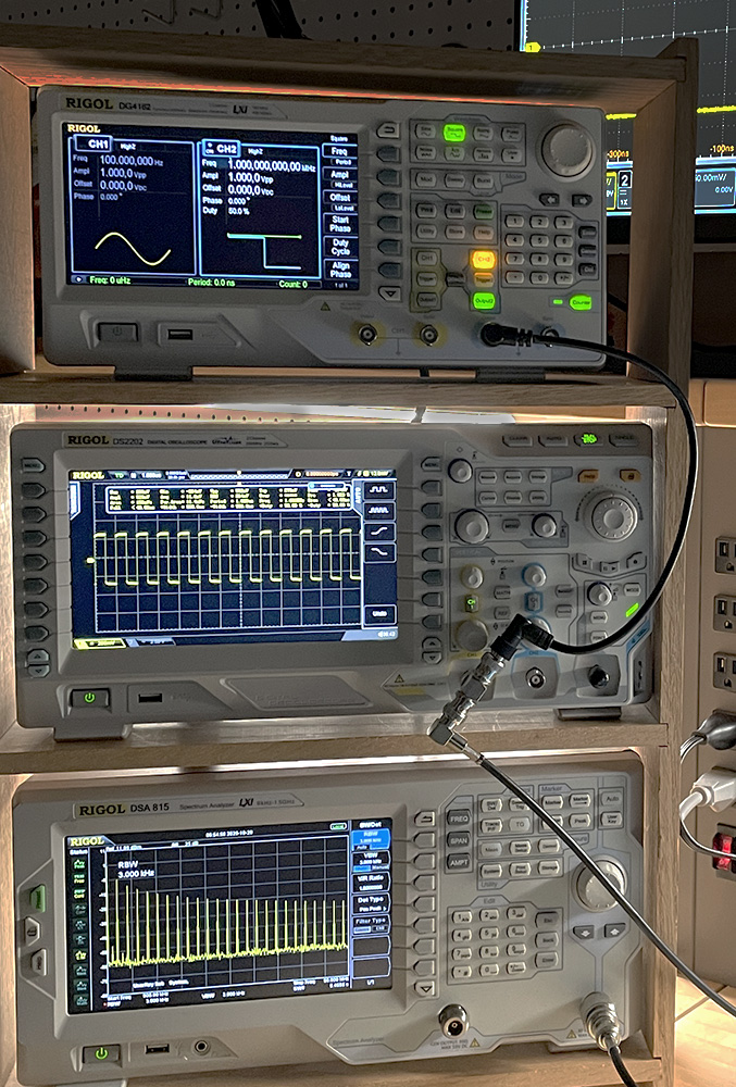
Conducted and radiated emissions measurements are usually made in the frequency domain. Therefore, it's important for EMC engineers to understand how various time-domain waveforms look when they are displayed in the frequency domain. This exercise gives students an opportunity to view several canonical waveforms in both domains. It also provides an opportunity to become familiar with various spectrum analyzer features and settings.
Preparation: Students should read Chapter 4 before starting this exercise. They should be familiar with the basic operation of traditional EMI test receivers with peak, quasi-peak, and average detectors.
Equipment Required:
- waveform generator
- oscilloscope with a bandwidth ≥ 500 MHz
- spectrum analyzer or EMI test receiver
Procedure:
Step 1: Connect the waveform generator to both the oscilloscope and the spectrum analyzer using coaxial cables and a T-connector. Use the 50-Ω input for the oscilloscope.
Step 2: Set the spectrum analyzer to view frequencies from 500 kHz to 15 MHz. Set the resolution bandwidth to 10 kHz.
Step 3: Set the waveform generator to produce a 1-MHz sine wave with a peak amplitude of 1 volt as displayed on the oscilloscope.
Step 4: Put a marker on the spike appearing at or near 1 MHz on the spectrum analyzer display. 1-volt peak is 0.707 Vrms, which is 117 dB(μV) or 10 dBm. Calculate the error in the displayed frequency (compared to the oscilloscope waveform) and express it as a percentage. Calculate the error in the displayed amplitude and express it in decibels.
Step 5: Change the frequency of the signal to 10 MHz. Repeat the calculations in Step 4.
Step 6: Adjust the waveform generator to produce a 1-MHz square wave. Note the amplitude of the first 15 harmonics and compare the measured values to the expected values.
Step 7: Adjust the waveform generator to produce a 1-MHz triangular wave. Note the amplitude of the first 15 harmonics and compare the measured values to the expected values.
Step 8: Adjust the waveform generator to produce a 500 ns rectangular pulse with a 1000 ns repetition rate. Note that this is a 1-MHz square wave. How do the amplitudes of the first 15 harmonics compare to the values in Step 6?
Step 9: Decrease pulse width to 480 ns. What happens to the amplitude of the even harmonics?
Step 10: Increase the upper frequency of the measurement to 50 MHz. You should be able to see a (sin x)/x pattern in the envelope of the harmonics. Where does the first null appear? Why?
Notes:
Depending on the characteristics of the waveform generator and analyzer, other waveforms could be investigated. If the receiver is an EMI test receiver, students can make quasi-peak and average measurements at one of the harmonic frequencies.
This lab exercise could also be performed using a digital oscilloscope with an FFT function. In that case, adjustments to the resolution bandwidth, reference level, and video bandwidth would be replaced by adjustments to the sampling frequency, displayed amplitude, and averaging functions. Note that the FFT calculation on an oscilloscope displays peak values of the harmonics, not the rms values displayed on a spectrum analyzer.