
Chapter 3 Lab Exercise: Common Impedance Coupling in a Ribbon Cable
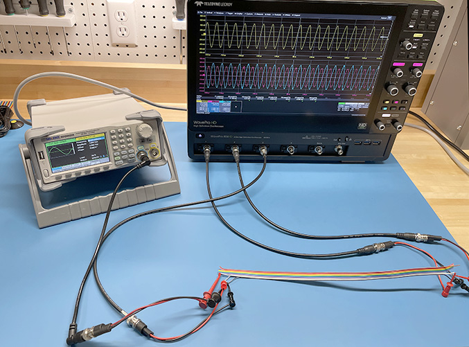
Ribbon cables are well-suited for crosstalk demonstrations and laboratory exercises. Two circuits sharing a return wire in a 50-cm ribbon cable exhibit measurable levels of all three types of EM coupling. The simple geometry of a ribbon cable allows students to calculate the expected amount of coupling and compare it to the measured coupling.
Preparation: Students should be provided with the dimensions of the ribbon cable and parameters of the test setup before coming to the lab. They should calculate the expected value of the common-impedance coupling before making any measurements. (This could be done as part of an earlier homework assignment.)
Equipment Required:
- RF signal source (100 Hz to 10 MHz)
- 3-channel oscilloscope
- 50-cm length of ribbon cable with at least 3 wires
Procedure:
Step 1: Connect the RF source to Channel 1 of the oscilloscope through wires 1 and 2 of the ribbon cable. Wire 1 should be connected to the grounded side of both instruments. Set the input impedance of Channel 1 to 50 Ω.
Step 2: Channel 2 of the oscilloscope should be connected to measure the voltage induced on another ribbon cable wire, preferably as far as possible from wires 1 and 2 (e.g., in a 9-wire ribbon cable, choose wire 9). The ground side of Channel 2 should be connected to wire 1 and the signal side to the other ribbon cable wire.
Step 3: Channel 3 of the oscilloscope should be connected to measure the voltage induced on the same wire as Channel 2 at the other end of the ribbon cable. Again, the ground side of Channel 3 should be connected to wire 1 and the signal side to the other ribbon cable wire.
Step 4: Starting at 100 Hz, increase the amplitude of the source until there are measurable sinusoidal waveforms on all three oscilloscope channels. Channel 1 will have a much higher amplitude than the other two channels. Channels 2 and 3 should display waveforms that are approximately the same amplitude, but 180° out of phase.
Step 5: Determine the ratio of the Channel 2 and 3 voltages to the Channel 1 voltage. How does this compare to the calculated value of the common-impedance coupling?
Step 6: Repeat the measurement above at 1 kHz, 10 kHz, 100 kHz, and 1 MHz. Compare to the calculated values of common-impedance coupling at those frequencies (be sure to account for the skin depth). Is the agreement good? If not, why not? Are the measured waveforms in Channel 2 and Channel 3 still equal in magnitude and 180° out of phase?
Step 7: If the signal source is a waveform generator, change the shape of the signal from a sine wave to a square wave. Describe the signal observed in Channels 2 and 3. Is this consistent with the expectation for common-impedance coupling? If not, why not?
Notes:
Using a battery-powered signal source and/or oscilloscope will prevent current from returning through the safety ground. In this case, the agreement between the measurements and calculations should be good at low frequencies. However, it can also be instructional to allow students to perform the measurements with grounded instruments. Engineers often learn more from results that don't agree with calculations than they learn from getting the expected result.
Students can try shorting wire 1 to other unused wires in the ribbon cable at both ends to reduce the resistance of the return path. Using two return wires instead of one should reduce the coupling by about 6 dB.
A key point of this exercise is to demonstrate that common-impedance coupling won't be the dominant coupling mechanism at high frequencies. At frequencies well above 100 Hz, the measured results won't agree with the common-impedance coupling calculations.