
The Fourier Series
Of course, many of the inputs to linear systems that we would like to analyze are not sinusoidal. In this case, it is desirable to represent time-domain signal waveforms as a sum of sinusoidal frequency components. In the frequency domain, each component can be analyzed individually. The frequency-domain system outputs can then be summed and converted back to the time domain.
A periodic signal can be represented as a sum of its frequency components by calculating its Fourier series coefficients. A periodic signal with period T can be written
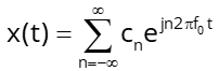 (1a)
(1a)
where f0 = 1/T and
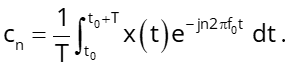 (1b)
(1b)
If x(t) is a real time-domain signal, the coefficients cn and c-n are complex conjugates (i.e., cn = c-n*) and we can rewrite Eq. (1a) in the form,
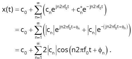 (2)
(2)
The Fourier series coefficients in this form consist of a DC component, c0, and positive harmonic frequencies, n2πf0 (n = 1, 2, 3, …). This is the one-sided Fourier series and the coefficients, 2|cn|, represent the peak value of each harmonic. Dividing the peak value by √2 yields the root-mean-square (rms) value. Signal harmonics measured with a spectrum analyzer or EMI test receiver are the rms values of the one-sided Fourier Series coefficients. In other words, the amplitude of each measured harmonic is √2|cn|.
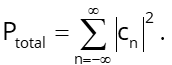
The frequency-domain representation of a periodic signal is a line spectrum. It can only have non-zero values at DC, the fundamental frequency, and harmonics of the fundamental. Because periodic signals have no beginning or end, non-zero periodic signals have infinite energy but finite power. The total power in the time-domain signal,
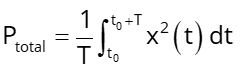 (3)
(3)
is equal to the sum of the power in each frequency-domain component,
 (4)
(4)
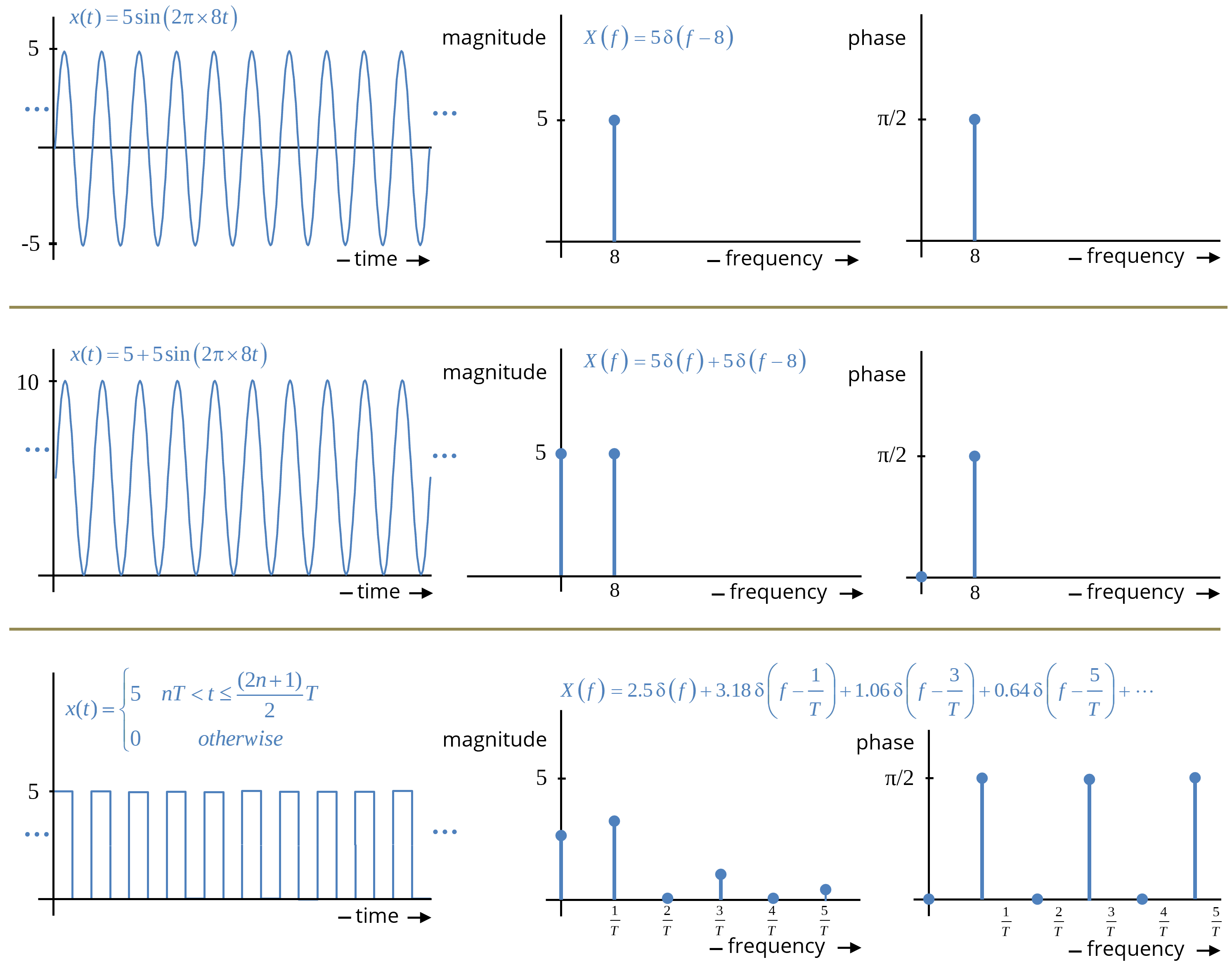
A few periodic signals and their frequency-domain representations are illustrated in Figure 1.
The Fourier Transform
Transient signals (i.e., signals that start and end at specific times) can also be represented in the frequency domain using the Fourier transform. The Fourier transform representation of a transient signal, x(t), is given by,
 (5)
(5)
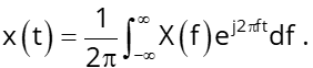
The inverse Fourier transform can be used to convert the frequency-domain representation of a signal back to the time domain,
 (6)
(6)
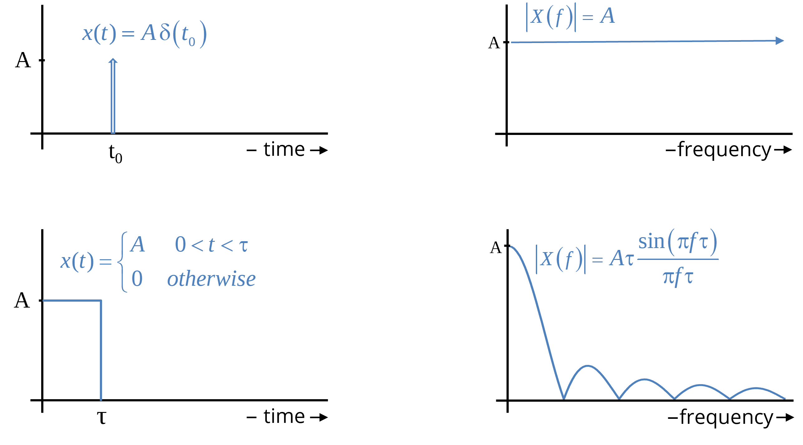
Two transient time-domain signals and their Fourier transforms are illustrated in Figure 2.
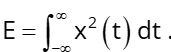
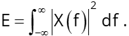
Note that transient signals have zero average power, when averaged over all time, but they have finite energy. The total energy in a transient time-domain signal is given by,
 (7)
(7)
This must equal the total energy in the frequency-domain representation of the signal,
 (8)
(8)