EMI Test Receivers

Traditional Spectrum Analyzer

A spectrum analyzer displays time-domain signals in the frequency domain. As illustrated in Figure 1, a traditional spectrum analyzer mixes (multiplies) the input signal with another sinusoidal signal generated by a voltage-controlled oscillator. The resulting signal has a frequency-domain representation identical to the original but shifted both up and down by an amount equal to the oscillator frequency. A band-pass filter captures power within a narrow frequency band as the voltage-controlled oscillator varies the amount of frequency shift over time. A plot of the band-pass filter’s output power versus the frequency shift provides a frequency-domain representation of the original signal.

Figure 1: Basic operation of a traditional spectrum analyzer.

A key parameter of this measurement is the bandwidth of the band-pass filter, called the resolution bandwidth. This bandwidth determines how finely individual frequencies can be resolved in the output.

Traditional spectrum analyzers can make accurate measurements over a wide range of frequencies, but they can also focus on specific narrow frequency bands to make high-resolution measurements.

Real-Time Spectrum Analyzer

A real-time spectrum analyzer also typically employs a mixer to down-convert the received signal to a lower frequency. As illustrated in Figure 2, the converted signal is then sampled using an analog-to-digital converter, and a Fast Fourier Transform (FFT) algorithm is used to convert the sampled time-domain signal to a sampled frequency-domain signal.

Overlapping time sequences are converted to the frequency domain, then digitally combined and displayed. The signal spectrum is continuously updated, allowing rapid changes in the spectrum to be monitored.

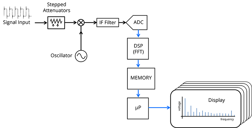
Figure 2: Basic operation of a real-time spectrum analyzer.

A significant advantage of time-domain spectrum analyzers is that they capture the entire signal content in a given frequency band all of the time. This allows the analyzer to capture brief transient events that a traditional spectrum analyzer might miss. Real-time spectrum analyzers are also generally faster and can trigger on events defined in the time or frequency domains.

Digital Oscilloscope

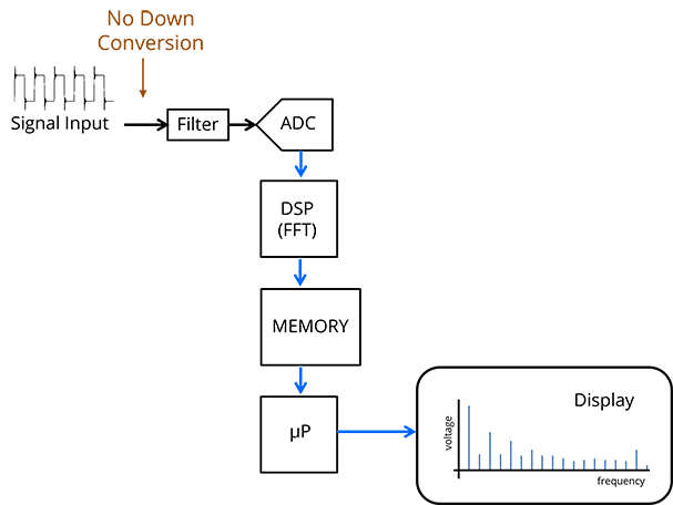
Figure 3: Basic operation of a digital oscilloscope with an FFT function.

Digital oscilloscopes with an FFT function can also display signals in the frequency domain. Modern scopes with sophisticated signal-processing algorithms can replicate many of the functions typically associated with spectrum analyzers. As indicated in Figure 3, digital oscilloscopes do not usually down-convert the received signal and are slightly more limited in their ability to display results in specific frequency ranges. On the other hand, a significant advantage of most digital oscilloscopes is their ability to process two input signals simultaneously on separate channels. This enables adding or subtracting signals (e.g., to determine common- and differential-mode components) or quantifying the correlation between two signals.

Digital oscilloscopes typically give users a lot of control over sampling parameters. The user needs to understand how changes in one parameter affect other important variables. Some of these relationships are listed in Table 1.

Table 1. Key Parameters for Time-Frequency Conversion using an FFT.

Peak, Quasi-Peak and Average Measurements

A spectrum analyzer measures the power in a given resolution bandwidth as a function of frequency. This power is typically expressed as an rms voltage across the 50-Ω input resistance of the test equipment and compared to a limit specified in the test specification. However, depending on the specification, the limit may apply to a measured peak value, a quasi-peak value or an average value. For example, the CISPR 32 conducted emissions specification, shown in Figure 4, places simultaneous limits on both the quasi-peak and the average values.

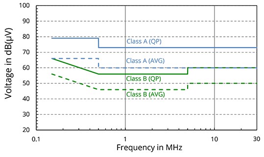
Figure 4: FCC and CISPR 32 conducted emissions limits.

A traditional spectrum analyzer with an envelope detector, as depicted in Figure 1, measures peak values (i.e., the highest rms voltage observed during the measurement dwell time). EMI test receivers are spectrum analyzers that can perform quasi-peak and average measurements using detectors that display a reduced amplitude for signals whose power at a given frequency fluctuates. Figure 5 illustrates how an intermittent signal results in different measured levels as detected by a peak, quasi-peak, and average detector.

Peak value: The peak value is the highest rms voltage observed in the given resolution bandwidth at the given frequency during the measurement window.

Average value: The average value is the rms voltage corresponding to the average power observed in the given resolution bandwidth at the given frequency during the measurement window. For example, if the signal is present 10% of the time and absent 90% of the time, the average value is 10 dB below the peak value.

Quasi-peak value: Quasi-peak detection was developed to quantify the amount of annoyance caused by repetitive pulsed noise sources. The quasi-peak value is determined by looking at the detector output as a function of time. When the signal is present, the detector output ramps up to the peak signal power with a specified attack time constant. When the signal is missing or has a lower amplitude, the detector output decays with a given decay time constant. The average value of the detector output is the quasi-peak value.

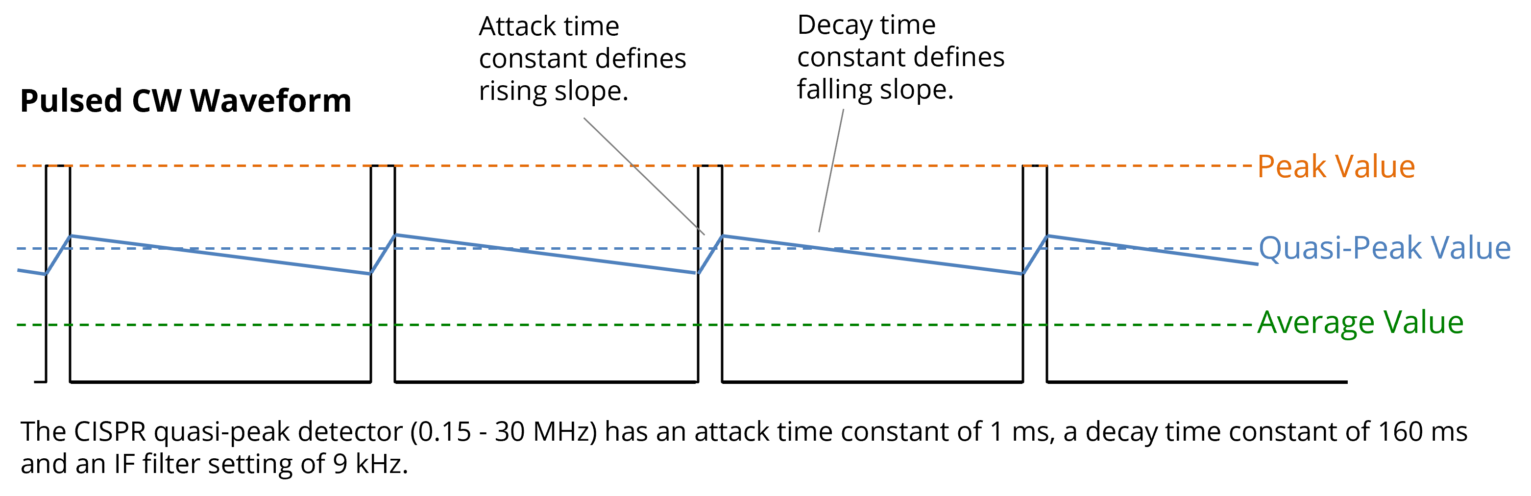
Figure 5: Response of peak, quasi-peak, and average detectors to an intermittent signal.

If the signal being measured is a series of brief impulses, a spectrum analyzer with a peak detector will record the energy detected in each impulse. This will correspond to the frequency and resolution bandwidth of the spectrum analyzer at the moment the impulse is detected. If the sweep time of the analyzer is 1 second, and pulses occur 100 times each second, then 100 narrowband frequency spikes will appear on the analyzer display with every sweep. In a max-hold mode, where the analyzer stores and displays the highest value observed over multiple sweeps, the impulsive noise will eventually have a non-zero value at every frequency in the measurement range. The measured spectrum will be broadband with an envelope corresponding to the Fourier transform of an individual impulse. However, because of the impulsive nature of the signal, the quasi-peak and average amplitudes will be considerably lower than the peak amplitude at any given frequency.

Circuits that illustrate how the various detectors in an EMI test receiver operate are shown in Figure 6. The output voltage of the peak detector is simply the rms amplitude of the rectified input. The quasi-peak detector output is essentially the voltage across a capacitor that charges with one time constant and discharges with a different time constant. The average detector is similar to the quasi-peak detector, but the charge and discharge time constants are the same.

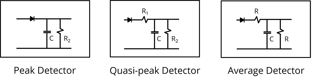
Figure 6: Simple representations of the detectors in EMI test receivers.

For impulsive noise sources with low repetition rates, the quasi-peak and average values will be much lower than the peak value. If the interval between impulses is shorter than the decay time of the detector, the quasi-peak and average values will increase with higher repetition rates.

Peak values are always greater than or equal to quasi-peak values, which are always greater than or equal to average values. All three values are the same for any signal that is always present with constant amplitude, or signals consisting of impulses with very high repetition rates.