
Crosstalk in Electrically Short Transmission Lines
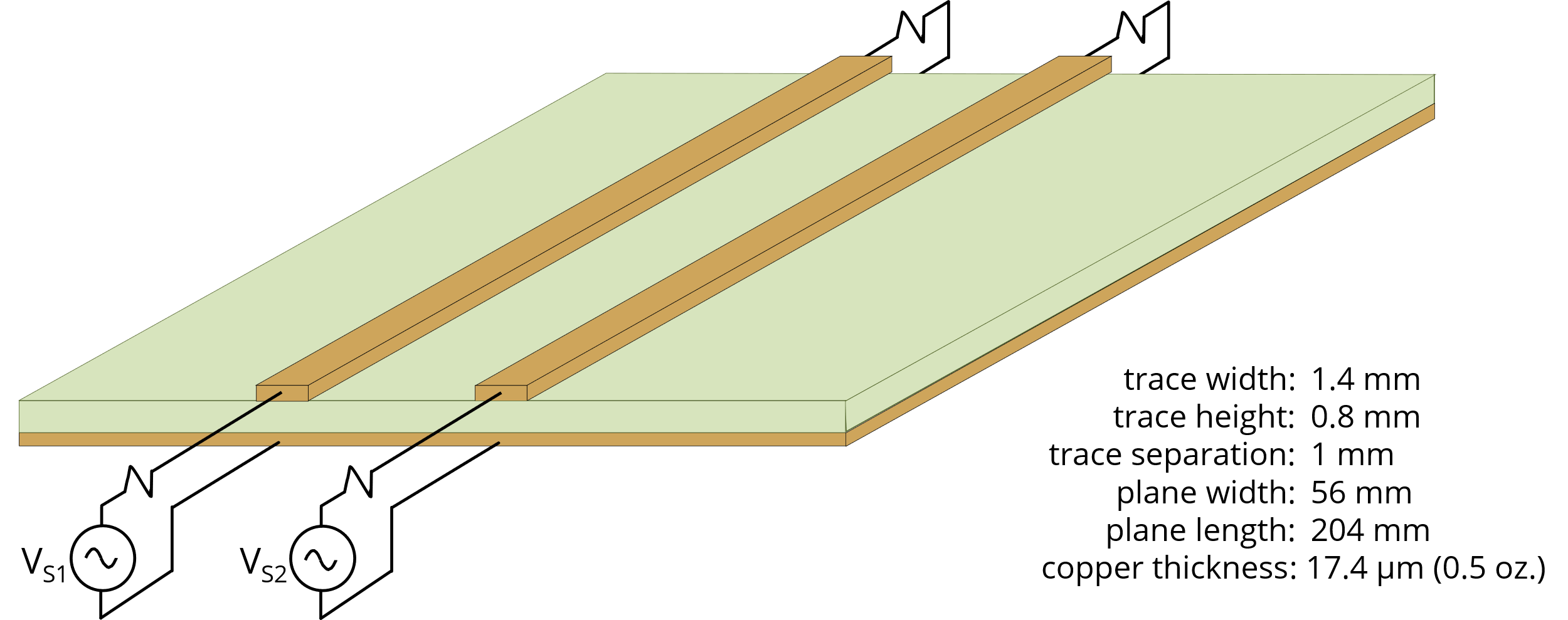
Figure 1. Two signal traces sharing a circuit board return plane.
Transmission lines that are short relative to a quarter-wavelength can generally be modeled using lumped-element parameters. In Chapter 3, the crosstalk for several different circuit configurations was calculated. Here, we’ll calculate the crosstalk between the pair of microstrip traces illustrated in Figure 1.
In this example, both traces carry signals from a 50‑Ω source to a 50‑Ω load. The trace width, height and separation are 1.4 mm, 0.8 mm, and 1 mm, respectively. The circuit board plane length and width are 204 mm and 56 mm, respectively. The copper (σ = 5.7 × 10⁷ S/m) is 17.4 µm thick. The effective relative permittivity of the dielectric is 4.2.
The voltage and current are approximately constant at frequencies where the traces are short relative to a quarter wavelength. At these frequencies, the traces can be modeled using lumped impedance parameters. For these calculations, we will make a weak-coupling assumption. That is, we will assume the coupling to the victim circuit does not significantly affect the voltages and currents in the source circuit. Virtually all practical cases of unintentional crosstalk involve weak coupling. However, when a weak-coupling assumption is made, and the calculated crosstalk is not weak (e.g., greater than -20 dB), a more precise calculation may be required.
Crosstalk Due to Common-Impedance Coupling
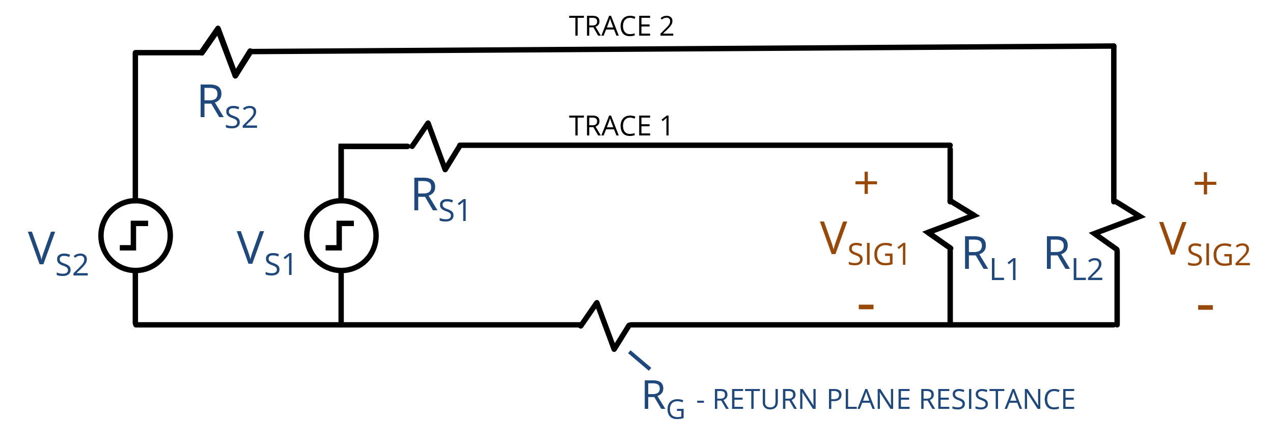
Figure 2. Circuits with a shared return resistance.
Figure 2 shows a schematic representation of the two trace circuits and their shared return-plane resistance. The crosstalk is the ratio of the induced voltage in the victim circuit (e.g., VSIG2) due to a signal voltage in the source circuit (e.g., VSIG1),
The voltage dropped across the return plane is approximately equal to the plane resistance times the Circuit 1 current, . A fraction of this voltage appears across the Circuit 2 source impedance, and the rest appears across the Circuit 2 load impedance. The voltage appearing at the load end contributes to the far-end crosstalk, which is calculated as
The voltage appearing across the source end contributes to the near-end crosstalk,
In this case, the resistance of the half-ounce copper return plane is,
The source and load impedances are all 50 Ω, so the magnitude of the crosstalk at either end due to common-impedance coupling is,
The victim circuit source and load impedances are the same, so the near-end and far-end crosstalk have the same magnitude. However, it’s worth noting that the coupled voltages at each end have opposite polarities.
In this example, the amplitude of the crosstalk is independent of frequency. This is generally true for common-impedance coupling unless the shared impedance is a function of frequency. At frequencies where the skin depth determines the value of the shared resistance, common-impedance coupling is generally proportional to the square root of the frequency (i.e., increases at a rate of 10 dB/decade).
The coupling can be proportional to frequency if the shared impedance is a small, lumped inductance or capacitance. However, in most cases, shared capacitances or inductances should be treated as electric-field or magnetic-field coupling, not common-impedance coupling.
A few properties of weak common-impedance coupling between electrically short transmission lines that are worth noting include the following.
- The coupling is proportional to the source circuit current.
- The coupling is usually independent of frequency.
- The near- and far-end coupling are 180° out of phase.
Crosstalk Due to Electric-Field Coupling
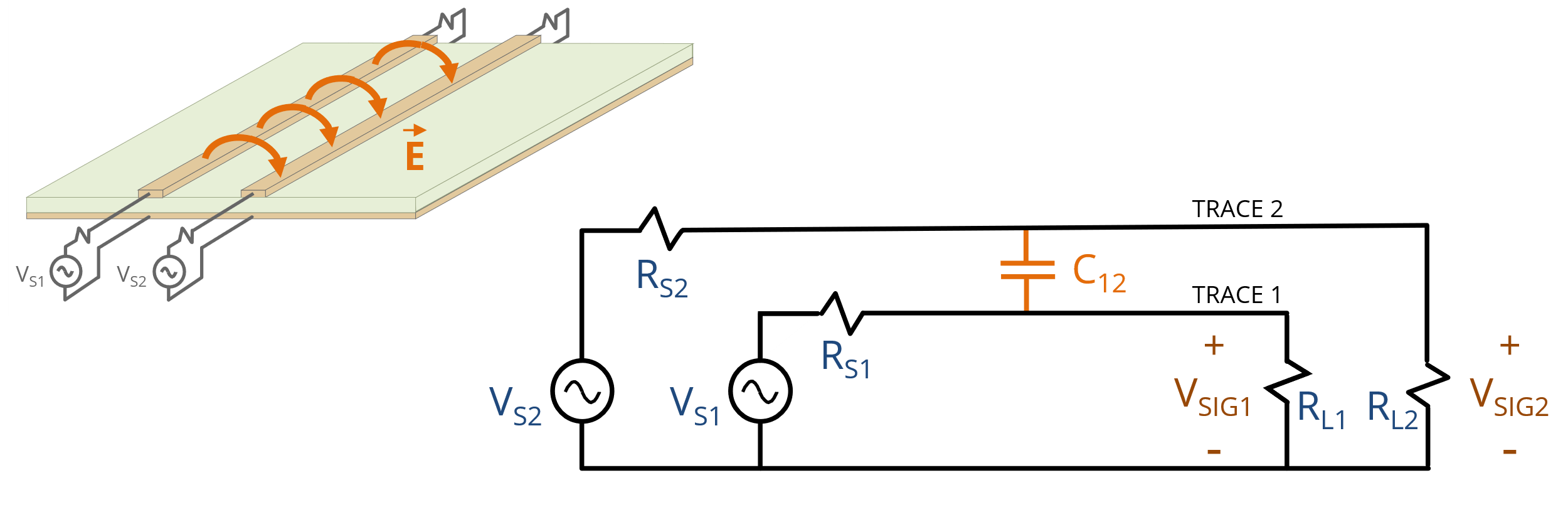
Figure 3. Electric-field coupling between traces.
Figure 3 shows a schematic representation of electric-field (capacitive) coupling between the two trace circuits. The electric-field coupling can be quantified using the mutual capacitance between the two traces. The crosstalk for this circuit can be calculated as
Or, making a weak-coupling assumption,
For the two traces illustrated in Figure 1, the mutual capacitance is 2.84 pF. Therefore, the calculated crosstalk at 10 MHz is
Note that the crosstalk is proportional to frequency, so at 20 MHz, it would be 6 dB higher (-41 dB). This is considerably stronger than the common-impedance coupling previously calculated for the same geometry (-89 dB). In this example, the electric-field coupling is higher than the common-impedance coupling at any frequency above about 8 kHz.
A few properties of weak electric-field coupling between electrically short transmission lines worth noting include the following.
- The coupling is proportional to the source circuit voltage.
- The coupling is proportional to frequency.
- The near- and far-end coupling have the same polarity.
Crosstalk Due to Magnetic-Field Coupling
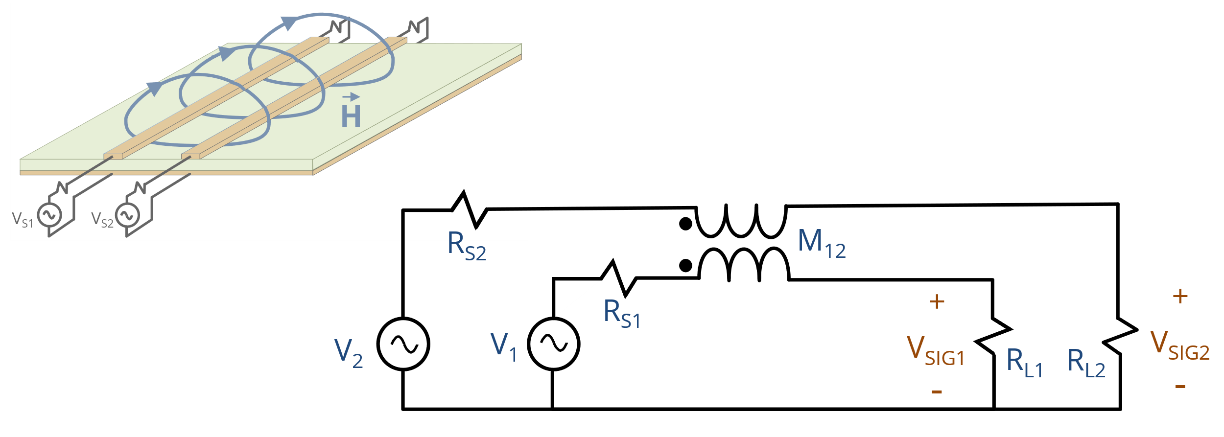
Figure 4. Magnetic-field coupling between traces.
Figure 4 shows a schematic representation of magnetic-field (inductive) coupling between the two trace circuits. The magnetic-field coupling can be quantified using the mutual inductance between the two trace circuits.
The far-end crosstalk for this circuit, making a weak-coupling assumption, is
where M12 is the mutual inductance between the two circuits and L22 is the self-inductance of the victim circuit. In most practical circuits, and that term can be neglected. Note that the total voltage coupled to the victim loop is proportional to . The term in parentheses expresses the fraction of the total voltage that appears across RL2. To calculate the near-end crosstalk, RS2 would replace RL2 in the numerator of that expression,
For the two traces illustrated in Figure 1, the mutual inductance is 16.4 nH. Therefore, the calculated far-end crosstalk at 10 MHz is,
Note that the crosstalk is proportional to frequency, so at 20 MHz, it would be 6 dB higher (-33.7 dB). This is about 7 dB higher than the electric-field coupling. In matched transmission lines with a homogeneous dielectric, the electric-field coupling and the magnetic-field coupling always have the same magnitude. However, in matched microstrip transmission lines such as this, magnetic-field coupling always dominates.
A few properties of weak magnetic-field coupling between electrically short transmission lines worth noting include the following.
- The coupling is proportional to the source circuit current.
- The coupling is proportional to frequency.
- The near- and far-end coupling are 180° out of phase.
Crosstalk Due to All Coupling Mechanisms
In unmatched electrically short transmission lines, one coupling mechanism is likely to dominate the overall crosstalk. However, in matched or nearly-matched lines, the magnitude of the electric- and magnetic-field coupling can be similar. At the far end, the coupled voltages due to the two field-coupling mechanisms are 180° out of phase. At the near end, the coupled voltages are in phase, and the total coupled voltage is the sum of the two.
For example, the total near-end crosstalk for the parallel trace configuration in Figure 1 is due to electric-field coupling (4.46 × 10⁻³) plus the magnetic-field coupling (10.3 × 10⁻³). Thus, the overall near-end crosstalk is 14.8 × 10⁻³ or -36.7 dB. The magnitude of the far-end crosstalk is the magnetic-field crosstalk (10.3 × 10⁻³) minus the electric-field crosstalk (4.46 × 10⁻³), which is 5.84 × 10⁻³ or ‑44.7 dB.
As indicated earlier, common-impedance coupling in circuit board return planes is unlikely to be a concern at frequencies above 100 kHz. The plane resistance is small (less than 1 mΩ per square for half-ounce copper planes). Also, return currents are largely concentrated near their respective signal traces. They will not share the same copper in the return plane unless the traces are vertically stacked above the same region of the plane.
Crosstalk in the Time Domain
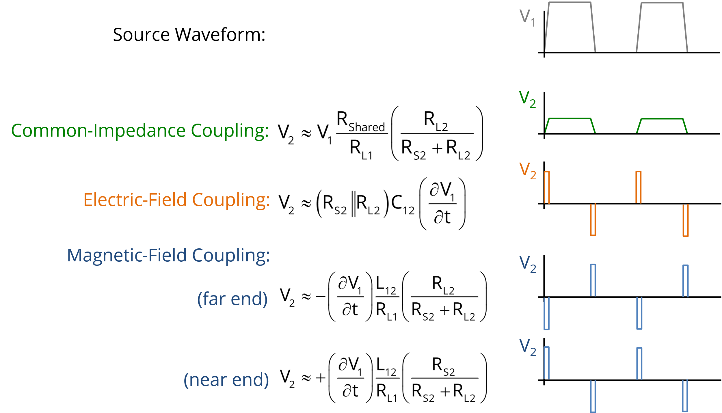
Figure 5. Time-domain crosstalk expressions for electrically short lines.
Time domain expressions for the crosstalk in electrically short transmission lines are easily obtained by substituting ∂V/∂t for ωV in the frequency-domain expressions. Note that although these expressions were derived in terms of voltage ratios, common-impedance coupling is proportional to the signal current and magnetic-field coupling is proportional to the time rate of change of the current . A summary of the time-domain expressions for crosstalk and a visual representation of the crosstalk from a trapezoidal waveform are provided in Figure 5. In each case, the weak-coupling assumption has been applied.
Example 6-1: Voltage Coupled from Digital Clock
Calculate the peak voltage coupled for the microstrip traces in Figure 1 when the source trace carries a 3.3-V, 10-Mbps digital signal with a 1‑ns transition time.
As indicated in Section 6.1.2, the mutual capacitance between the two traces is 2.84 pF. So, the peak coupled voltage due to electric-field coupling is,
As indicated in Section 6.1.3, the mutual inductance between the two traces is 16.4 nH. So, the peak coupled voltage due to magnetic-field coupling is,
Note that the magnetic-field coupling has the same amplitude at both ends, with opposite polarity. At the far end, the electric and magnetic-field coupling have opposite polarities, so the total coupled voltage is,
At the near end, the total coupled voltage is,
The coupled voltage due to common-impedance coupling is much lower than the field-coupled voltage. The DC calculation is the same in either the time or frequency domain,
Note that the common-impedance coupling calculation in the example above used the low-frequency value of the plane resistance, ignoring the skin effect. Since skin depth depends on frequency, applying it in the time domain is not straightforward. Nevertheless, at frequencies where the skin effect is important, the return currents on a plane will be concentrated under their respective traces, and any common-impedance coupling is generally negligible compared to the field coupling.