
Crosstalk in Electrically Long Transmission Lines
In short transmission lines, the crosstalk was proportional to the length of the lines. However, the crosstalk does not increase indefinitely with length. Two things can happen that limit the amount of crosstalk as the lines get longer.
For some tightly-coupled lines, the weak-coupling assumption may be violated. At this point, the source circuit becomes noticeably loaded. If the lines remain electrically short, lumped-element circuit models can be used to determine the coupled voltage, but the simple equations provided in the previous section no longer apply.
For all coupled transmission lines, when their length is no longer short relative to a quarter wavelength, voltage and current on the line are a function of position, and simple lumped-element models can no longer be applied.
Most practical transmission lines are not coupled strongly enough to violate the weak-coupling assumption. However, the second situation is common. Crosstalk between high-speed data communication signals is often strongest at frequencies where the lines are not electrically short. Transmission lines that are not electrically short should be matched. Therefore, it is important to be able to calculate the crosstalk between long, matched transmission lines.
Electric-Field Coupling in Long Lines

Figure 1. Lumped element model of electric-field coupling.
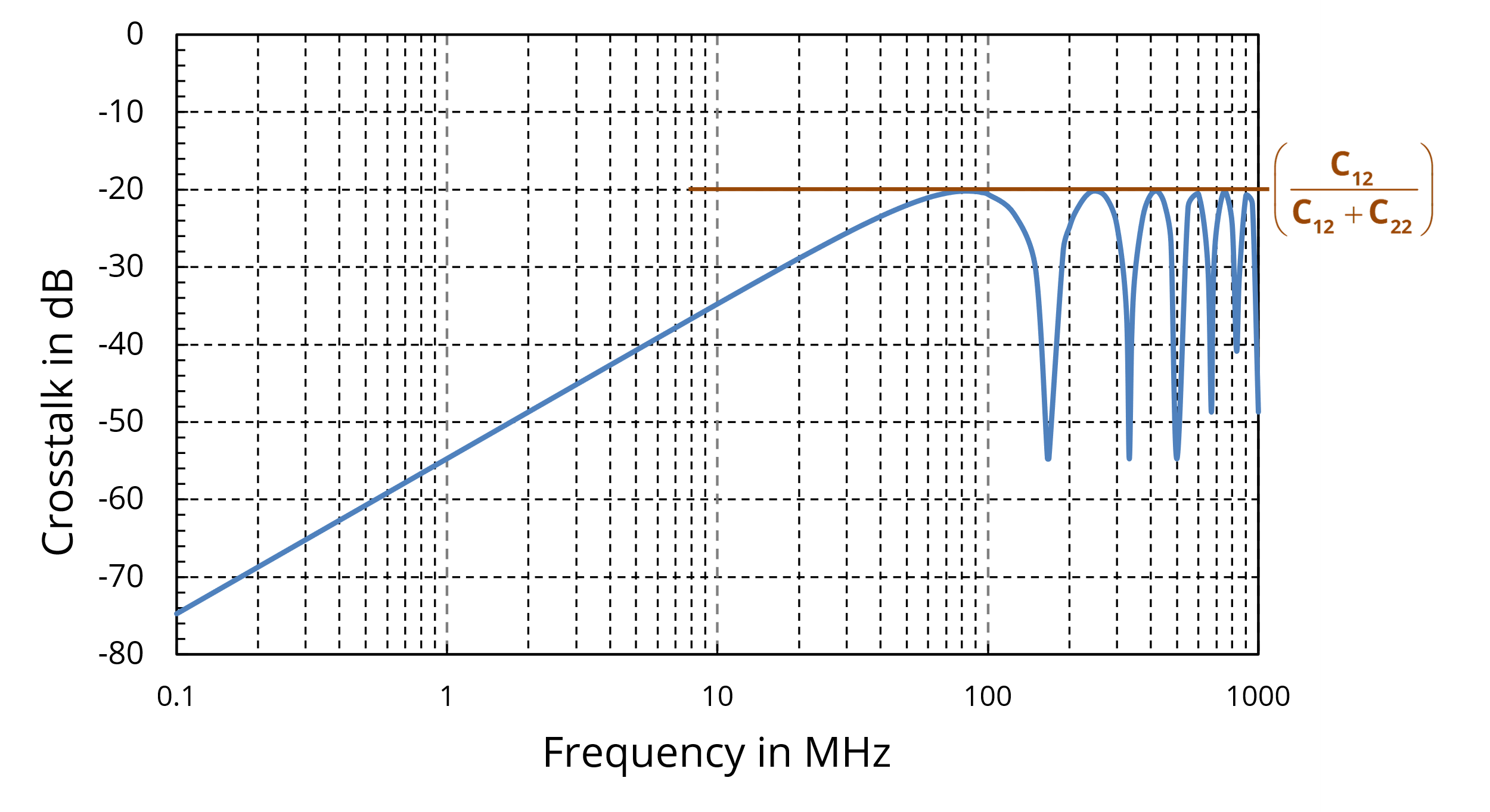
Figure 2. Far-end crosstalk between two matched transmission lines due to E-field coupling.
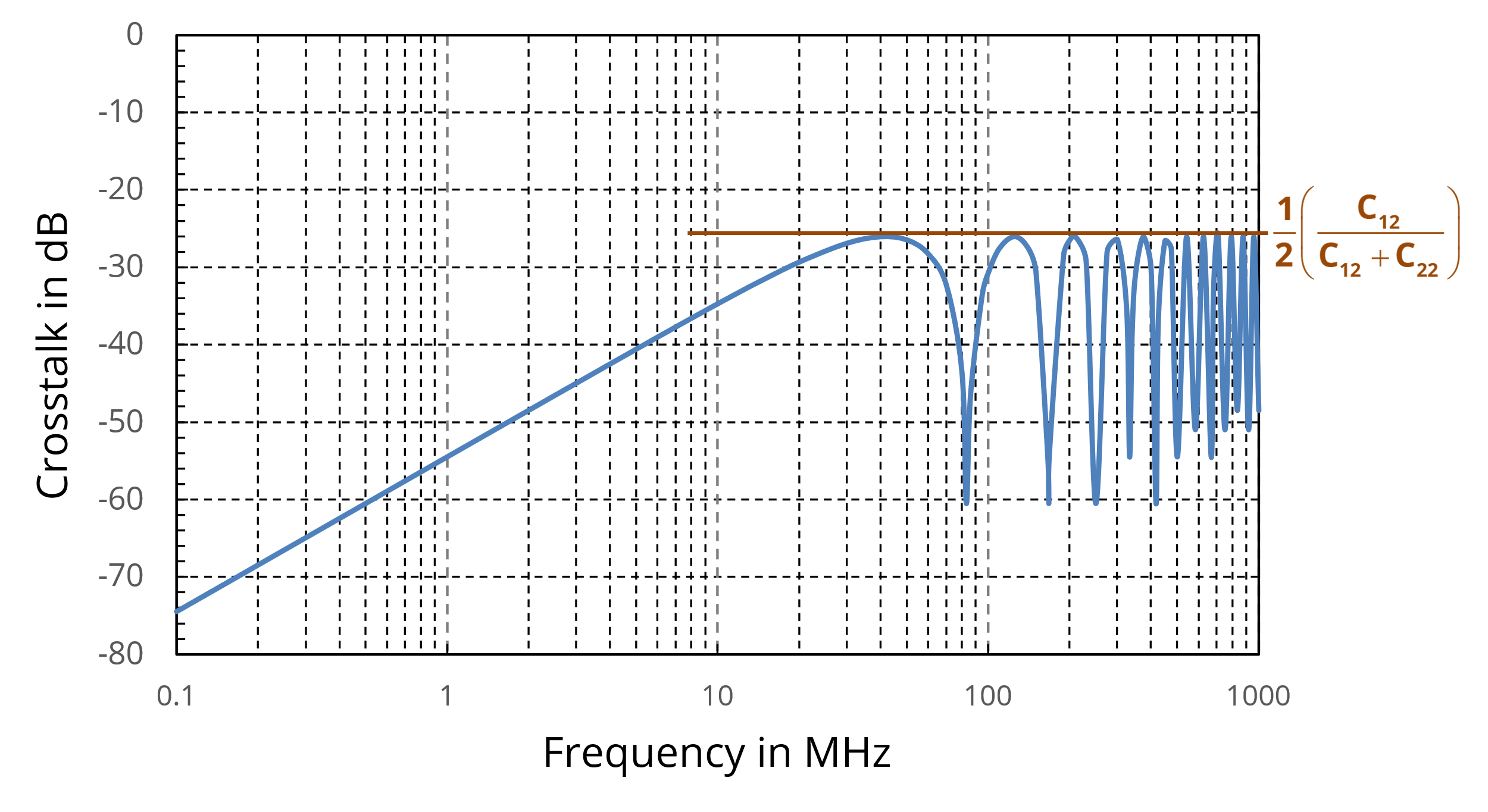
Figure 3. Near-end E-field crosstalk between matched transmission lines.
Let’s start by examining the electric-field coupling in a long transmission line that is matched at both ends. Figure 1 shows a schematic illustration of the geometry including segmented capacitances that couple the two lines. The brown line illustrates the voltage distribution along the source line at an instant in time.
To calculate the total far-end electric-field coupling, the contributions of each segment can be added. In the limit as the segment lengths approach zero, this summation is expressed as the integral,
Note that Z02 is the characteristic impedance of the victim transmission line. The last step in this calculation takes advantage of the fact that . Figure 2 plots the calculated electric-field coupling between two 50-cm transmission lines (Z01 = Z02 = 50 Ω, v = 1.67 × 10⁸ m/s). Note that the crosstalk reaches its peak value when the line length is an odd multiple of a quarter wavelength. In this case, the mutual capacitance between the lines is C12 = 13 pF/m, and the self-capacitance of the victim line is C22 = 120 pF/m. Therefore, the peak crosstalk is,
The calculation of the total electric-field coupling at the near-end is slightly different. The coupling from each segment does not build uniformly as the signal propagates. Instead, the near-end coupling from each segment propagates back towards the source, so the distance traveled is 2x instead of l‑x. The expression for the near-end coupling is therefore,
Figure 3 shows a plot of the calculated near-end electric-field coupling between the same two transmission lines. Note that the near-end crosstalk reaches its peak value when the length of the lines is an odd multiple of an eighth wavelength and its peak value is half that of the far-end crosstalk.
Magnetic-Field Coupling in Long Lines
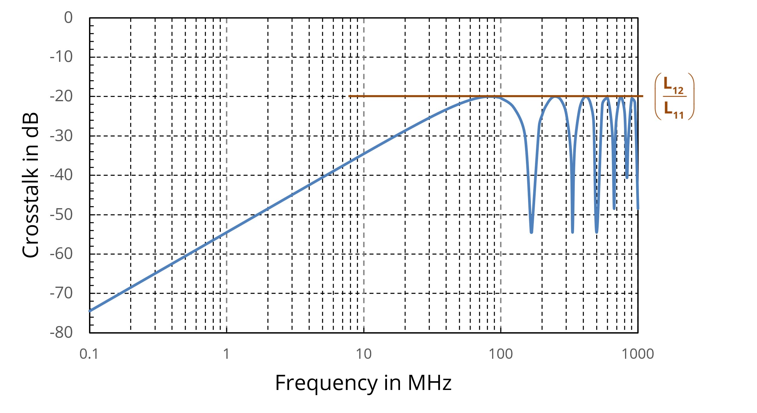
Figure 4. Far-end H-field crosstalk between matched transmission lines.
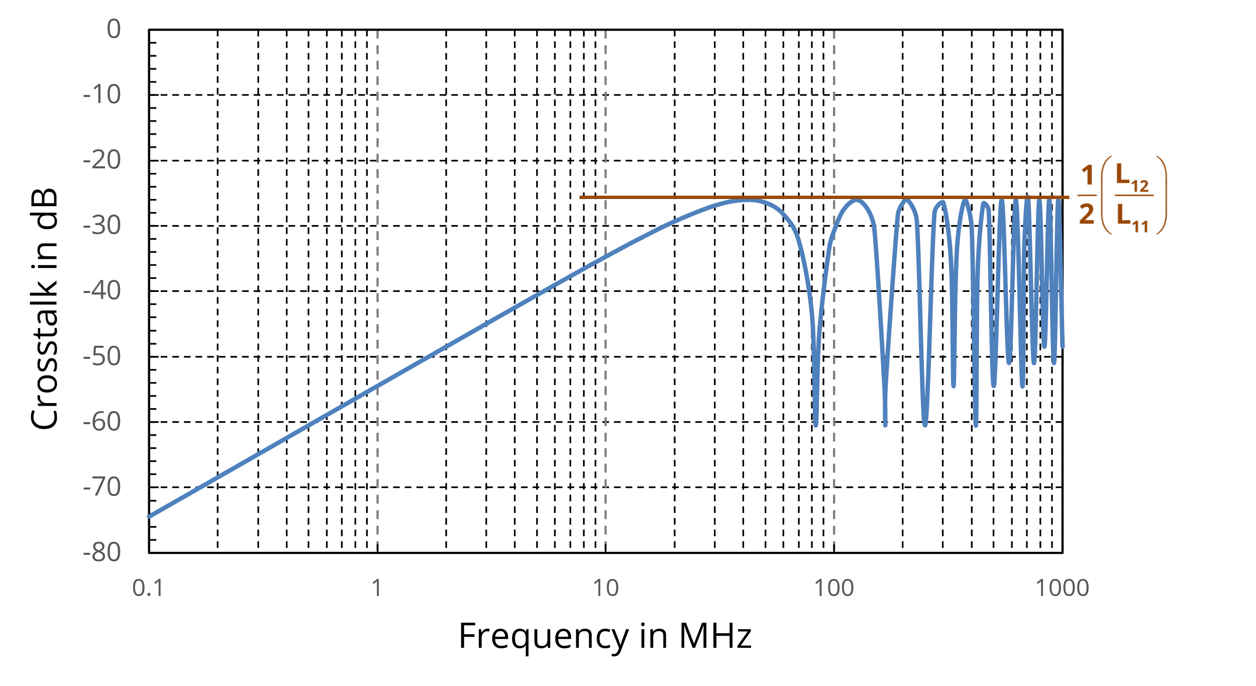
Figure 5. Near-end H-field crosstalk between matched transmission lines.
A calculation similar to (1) can be done to determine the total magnetic-field coupling.
Figure 4 plots the calculated magnetic-field coupling between two 50-cm transmission lines (Z01 = Z02 = 50 Ω, v = 1.67 × 10⁸ m/s). Note that the magnitude of the crosstalk in this plot equals the magnitude of the crosstalk due to electric-field coupling. In this case, the mutual inductance between the lines is L12 = 30 nH/m, and the self-inductance of the victim line is L22 = 300 nH/m.
For two transmission lines in a homogeneous dielectric, the magnitude of the electric- and magnetic-field coupling will always be the same. At the far end, the polarities are opposite, and the electric-field coupling will cancel the magnetic-field coupling. At the near end, the polarities are the same, and the contributions from each coupling mechanism will add. The calculation of the near-end magnetic-field coupling is similar to that in (3),
Figure 5 plots the calculated near-end magnetic-field coupling between the example transmission lines. Note that it is identical to the near-end electric-field coupling. This is because the ratio L12/L11 is equal to the ratio C12/(C12+C22) in a homogeneous dielectric.
Total-Field Coupling in Long Lines
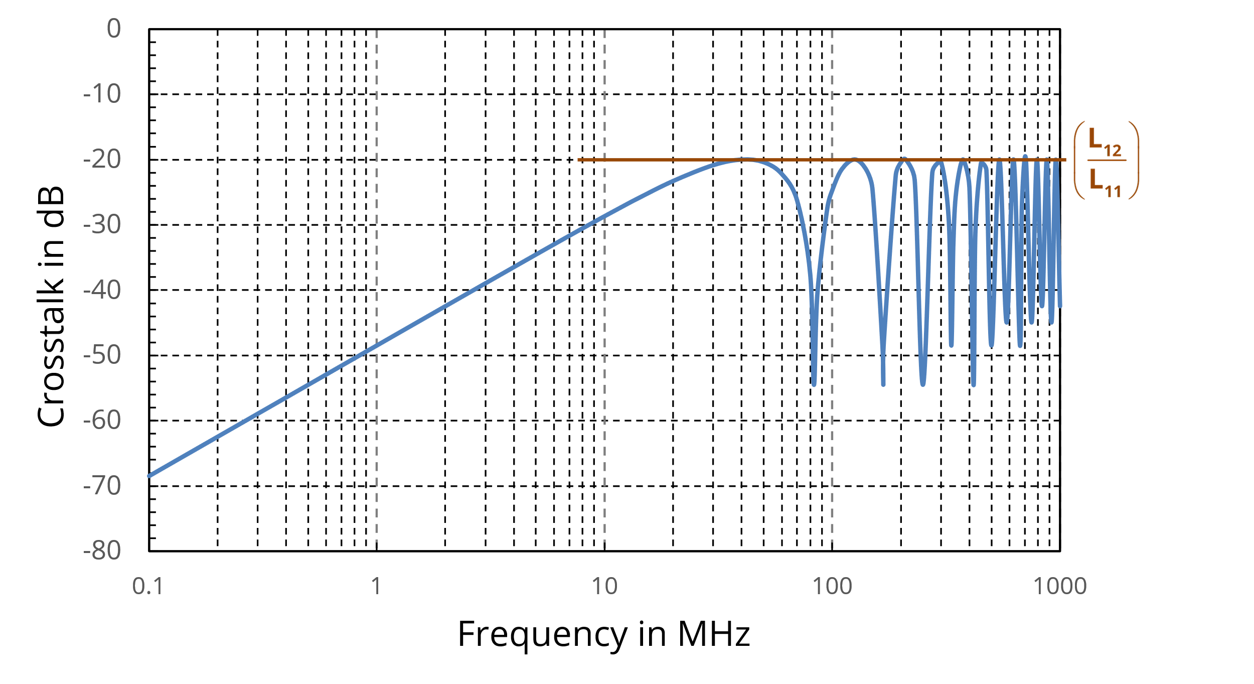
Figure 6. Total near-end crosstalk between matched transmission lines.
In a homogeneous dielectric, the electric- and magnetic-field coupling at the near end are equal in magnitude and add in phase. In this case, the total field coupling is twice the electric- or magnetic-field coupling. For the transmission lines in this example, the total near-end field coupling is plotted in Figure 6.
In a homogeneous dielectric, the electric-field and magnetic-field coupling at the far end cancel each other. In other words, no voltage is coupled to the far-end. All the coupled voltage appears at the near end. This is basically how a directional coupler works.
If the dielectric is not homogeneous, for example, in a microstrip trace geometry, the two types of field coupling are not necessarily equal. In coupled microstrip traces, magnetic-field coupling will be stronger than electric-field coupling. In this case, the total far-end crosstalk is the crosstalk due to the magnetic-field coupling minus that due to the electric-field coupling.
Crosstalk in the Time Domain
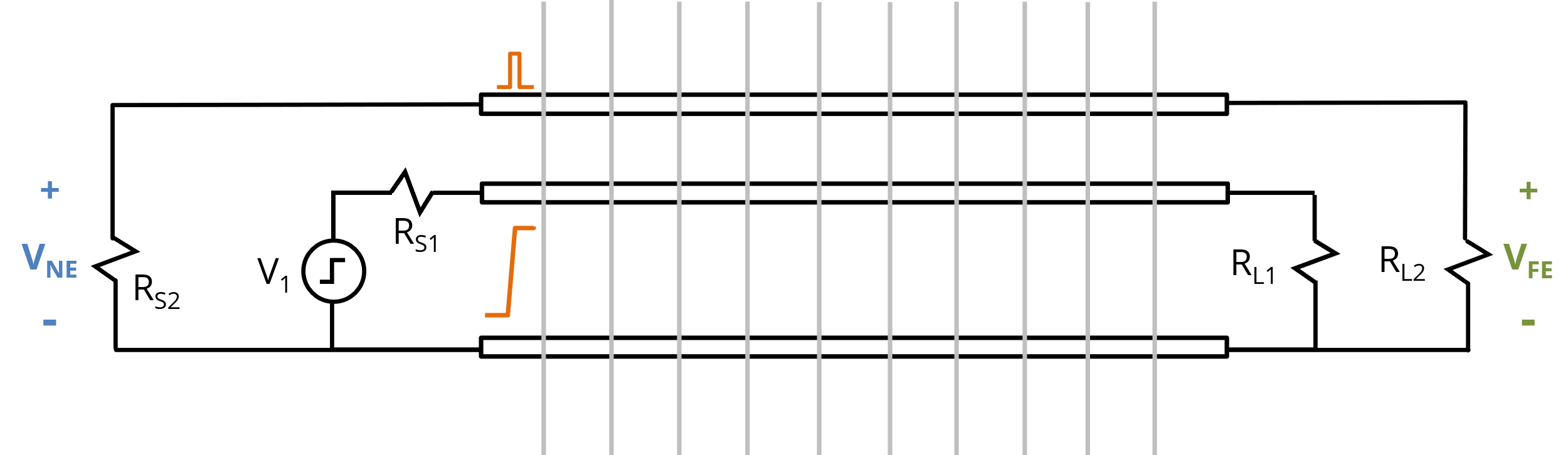
Figure 7. Initial crosstalk just after a source transition.
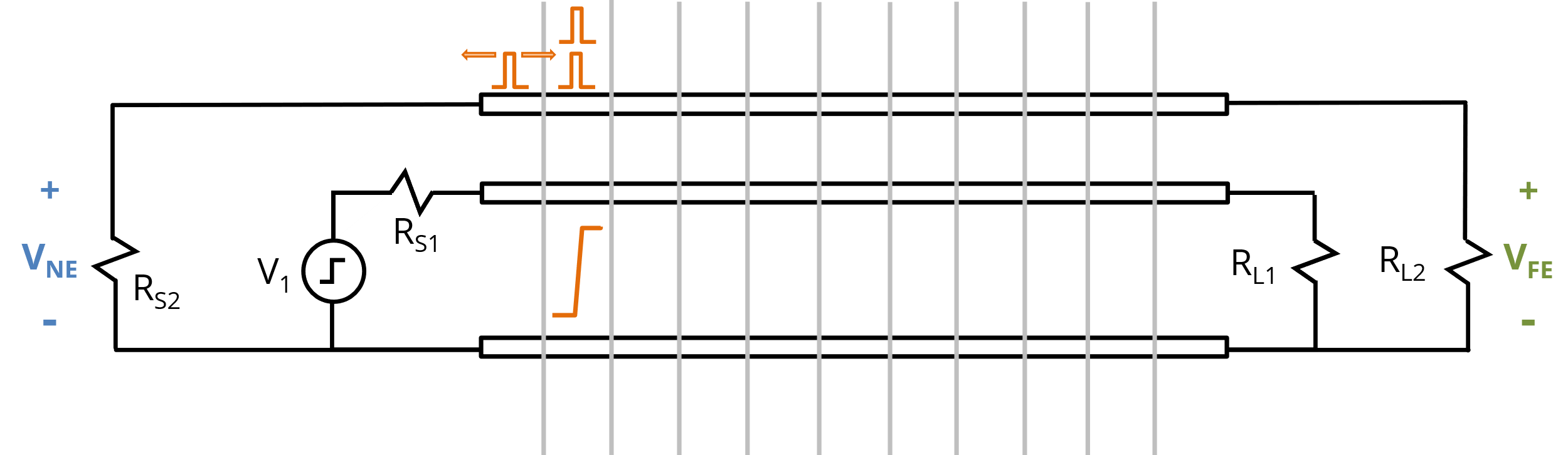
Figure 8. Crosstalk as the voltage transition begins to move down the line.
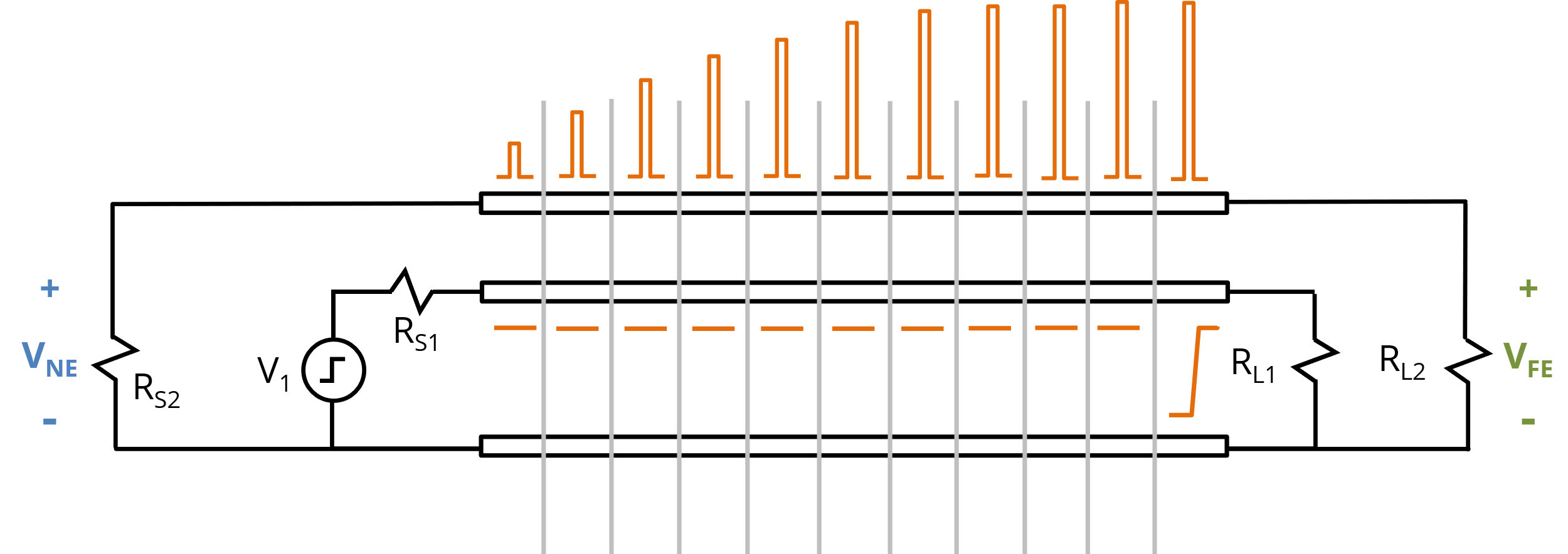
Figure 9. Crosstalk as the voltage transition reaches the end of the line.
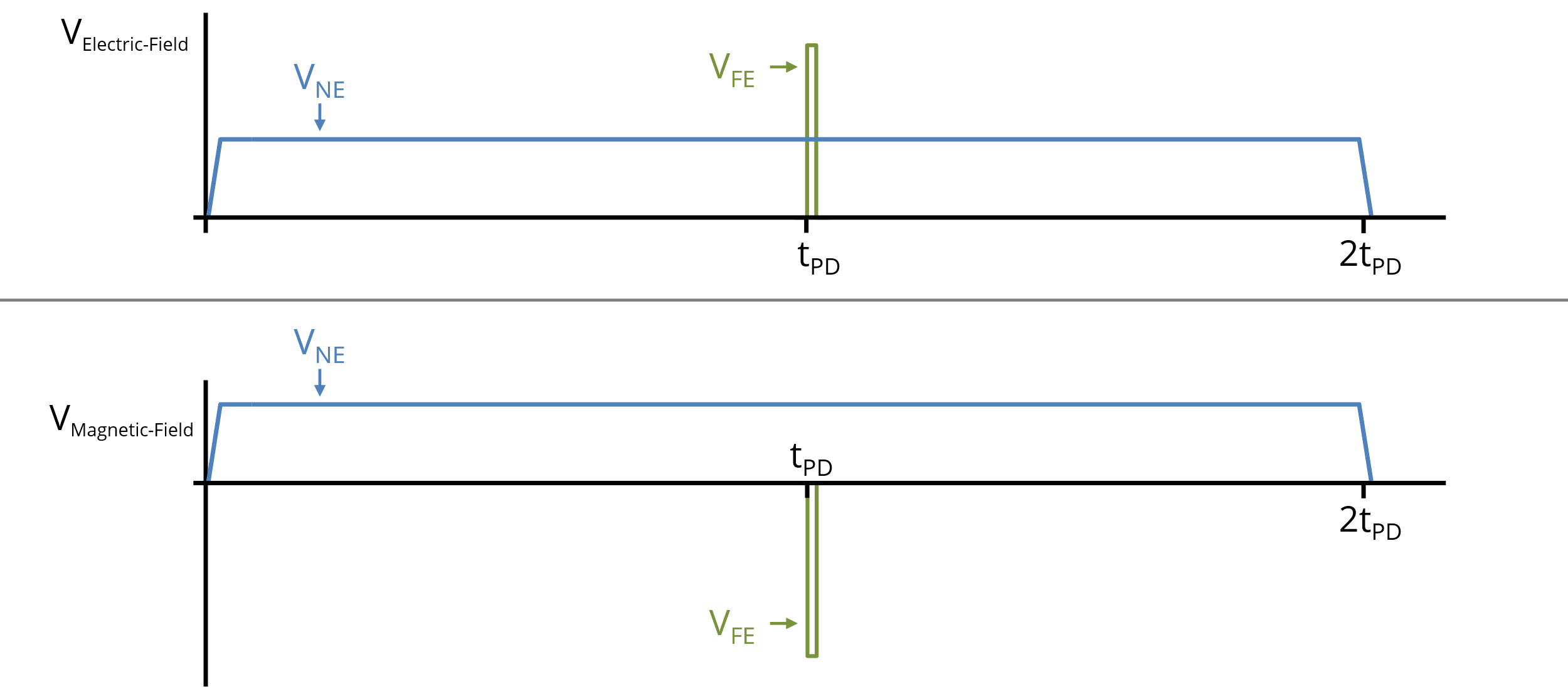
Figure 10. Near-end and far-end crosstalk for E-field and H-field coupling.
To understand how crosstalk looks in the time domain for electrically long lines, it’s helpful to view the lines as a series of electrically short segments. As illustrated in Figure 7, a step transition in the first segment of one line induces a spike in the first segment of the coupled line. For the electric-field coupling, the spike is an injected current with an amplitude of equation, where C is series combination of C12 and C22 multiplied by the length of the first short segment.
The injected current splits into a component that moves backward towards the near end, and a component that moves forward toward the far end of the transmission line. A short time later, the transition in the source line has moved to the second segment, as illustrated in Figure 8. Here, it couples to the second segment of the victim line. However, this segment also receives the spike coupled to segment 1 of the victim trace. The sum of the two produces a spike in the second segment of the victim trace that is about twice as strong as the spike in the first segment.
As the step transition continues to move down the source line, it couples more voltage to the victim line. As the coupled spike grows, its voltage limits the amount of electric-field coupling. Eventually, the spike amplitude reaches a steady-state value and stops growing, as indicated in Figure 9. The voltage (due to electric-field coupling) observed across the load at the far end is a single spike. For two identical lines matched at both ends, the maximum amplitude of the coupled spike is equation.
At the near end, the short spike coupled from the first segment arrived right away, followed by spikes with the same amplitude from subsequent segments. In the limit, as the segment lengths approach zero, there is a constant stream of new spikes, resulting in a coupled voltage waveform with a constant value. For two identical lines matched at both ends, the maximum amplitude of the coupled spike due to electric-field coupling is .
The coupled voltage waveforms at the near end, VNE, and the far end, VFE, due to electric-field coupling are shown in the top plot in Figure 10. The near-end waveform is a constant-voltage pulse with a duration twice the propagation delay. The far-end voltage is a spike arriving at a time equivalent to one propagation delay.
The magnetic-field coupling between two identical matched lines is plotted in the lower half of Figure 10. The near-end crosstalk has the same shape as the electric-field coupling and an amplitude . The far-end crosstalk is a spike with opposite polarity relative to the electric-field coupled voltage and an amplitude .
The total crosstalk is the sum of the electric- and magnetic-field coupling. These components add in-phase at the near end. At the far end, they have opposite polarities, and the coupled voltage is the electric-field-coupled voltage minus the magnetic-field-coupled voltage.
In a homogeneous dielectric, the electric- and magnetic-field coupling have the same magnitude. If the transmission line is matched at both ends, the far-end components cancel, and there is no crosstalk at the far end. The near-end crosstalk has the shape shown in Figure 10, and an amplitude equation. If the transmission line is only matched at the far end, some of the near-end crosstalk is reflected, and the reflected waveform appears at the far end.
Modeling Crosstalk in SPICE
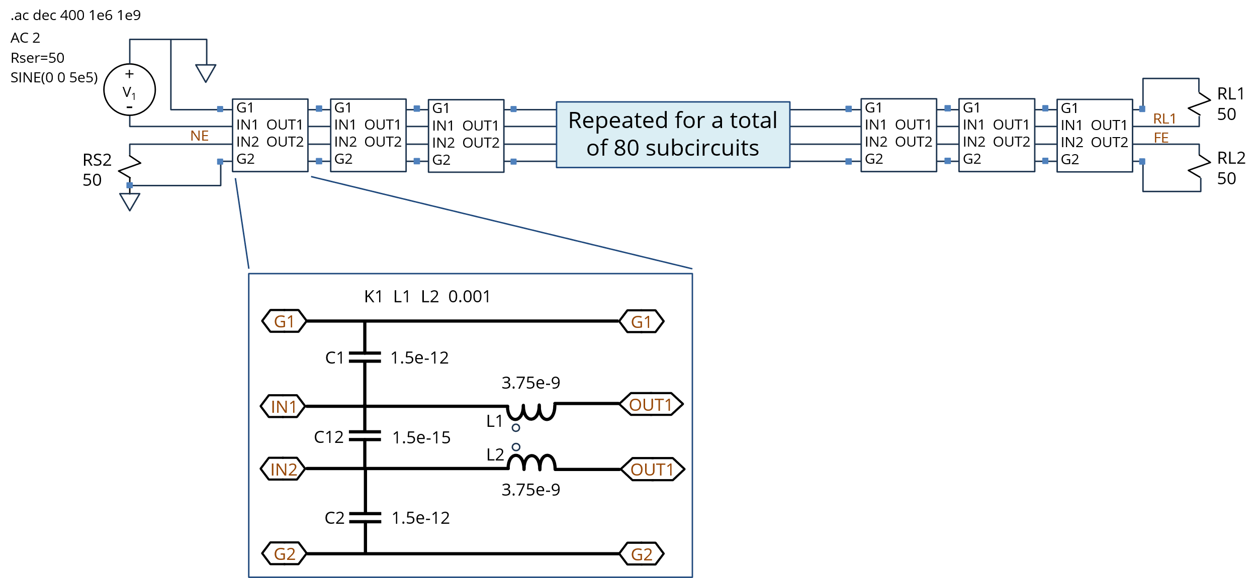
Figure 11. SPICE Model of coupled transmission lines with 80 LC sections.
Crosstalk can be accurately modeled with circuit simulators if the lumped-element parameters of the transmission lines are known. A common simulation approach uses 2D field simulators to obtain the per-unit-length RLCG parameters and SPICE to calculate the crosstalk.
Figure 11 shows a SPICE model for a pair of coupled, lossless transmission lines. The model is constructed with 20 sub-elements. Each sub-element has four lumped-element sections, yielding a total of 80 lumped-element sections from end to end. In this model, the capacitance per unit length of both lines is 120 pF/m. The inductance per unit length is 300 nH/m, yielding a characteristic impedance of 50 Ω and a propagation velocity of 1.67 × 10⁸ m/sec. To model a 1-meter length with 80 elements, each element has a capacitance of 1.5 pF and an inductance of 3.75 nH. The mutual capacitance modeled in each section is 1.5 fF, and the mutual inductance is 3.75 pH.
Figure 12 shows the calculated crosstalk as a function of frequency from 1 to 1000 MHz. Both transmission lines are matched. As expected, the near-end crosstalk rises at a rate of 20 dB/decade until the line length approaches a quarter wavelength, where it reaches its peak value of -60 dB (i.e., L12 / L11).
The calculated far-end crosstalk is very small, but it is not zero. This is a consequence of trying to calculate very small values using numerical inputs that are accurate to 2 or 3 significant figures. Changing the value of the mutual capacitance from 1.5 fF to 1.5015 fF, the calculated far-end crosstalk drops below -120 dB over the entire frequency range.
Figure 13 shows the calculated crosstalk when coupling coefficient is 10-2. Once again, the calculated far-end crosstalk is non-zero. In this case, the coupling is strong enough to change the characteristic impedance of both lines slightly. Replacing the 50-Ω terminations with 49.75-Ω terminations reduces the calculated far-end crosstalk below -120 dB over the entire frequency range.
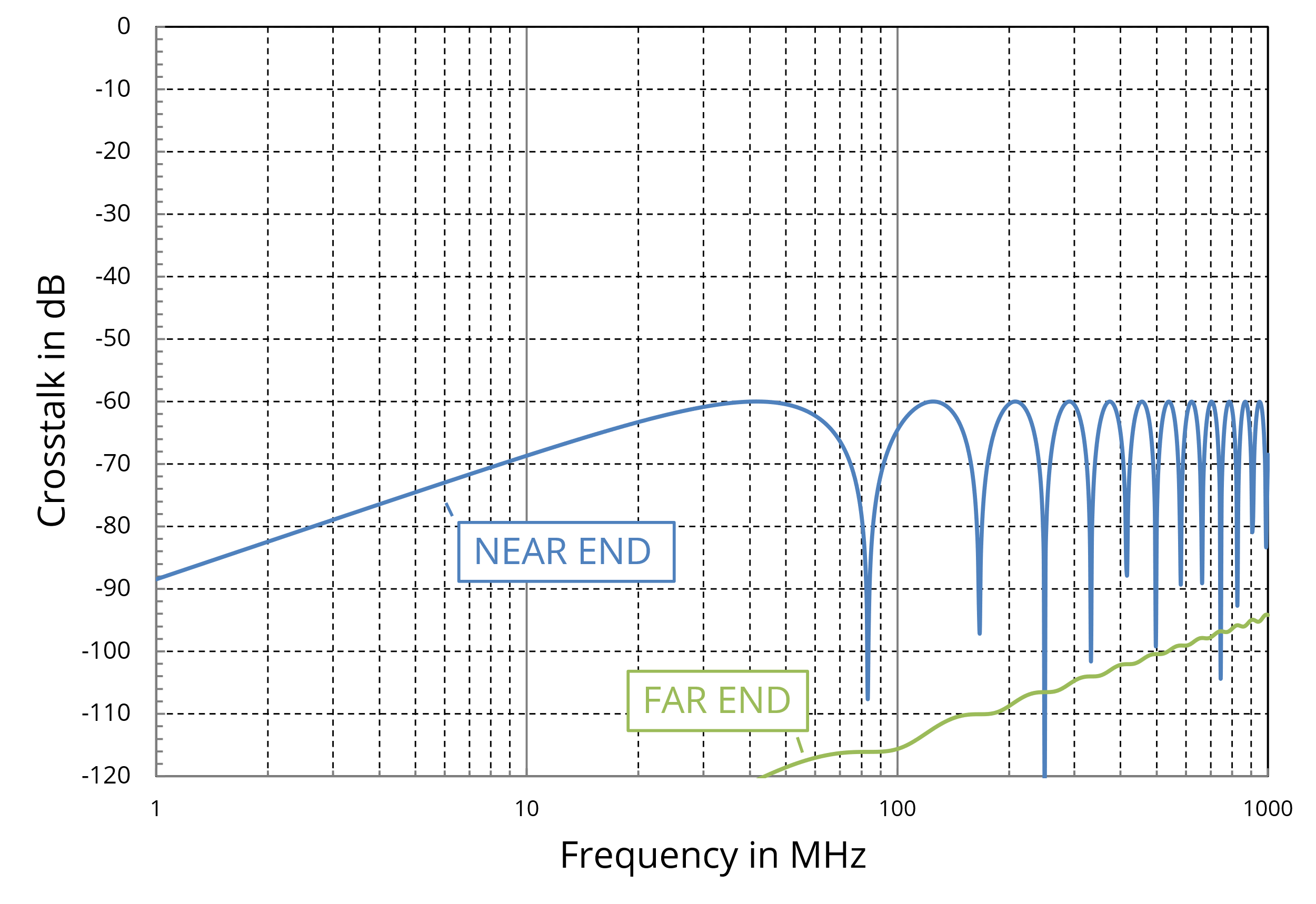
Figure 12. Crosstalk between two lines with L12/L11 = 10-3.
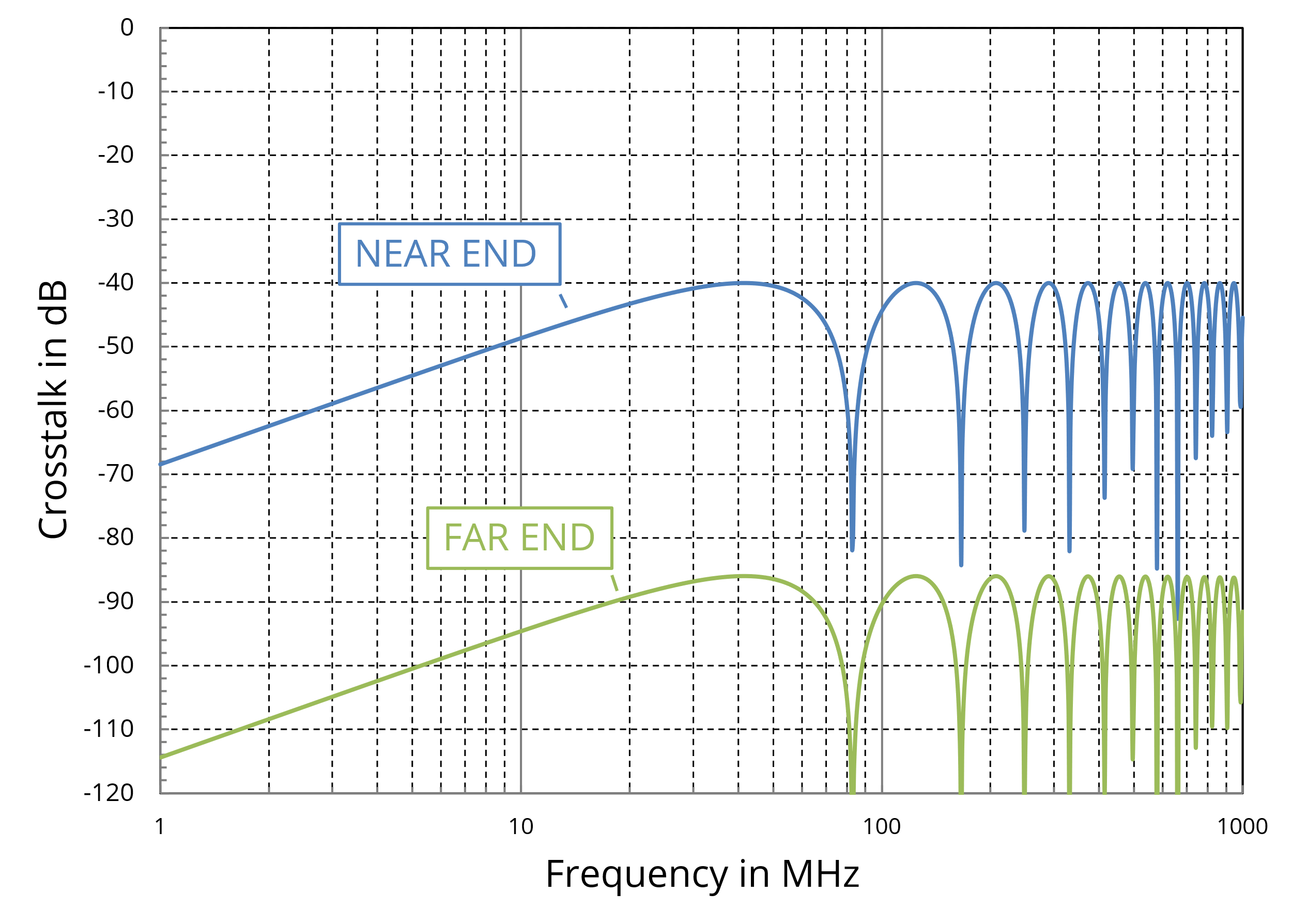
Figure 13. Crosstalk between two lines with L12/L11 = 10-2.
Figure 14 illustrates what can happen with an inhomogeneous dielectric. In this simulation, the E-field coupling coefficient, C12 / (C12+C22), is 0.009. The magnetic-field coupling coefficient is still 0.010. At the lower frequencies, the electric- and magnetic-field coupling nearly cancel at the far end. The far-end crosstalk is 26 dB lower than the near-end crosstalk. However, instead of leveling off at -40 dB, the far-end crosstalk continues to increase and eventually becomes the dominant coupling mechanism.
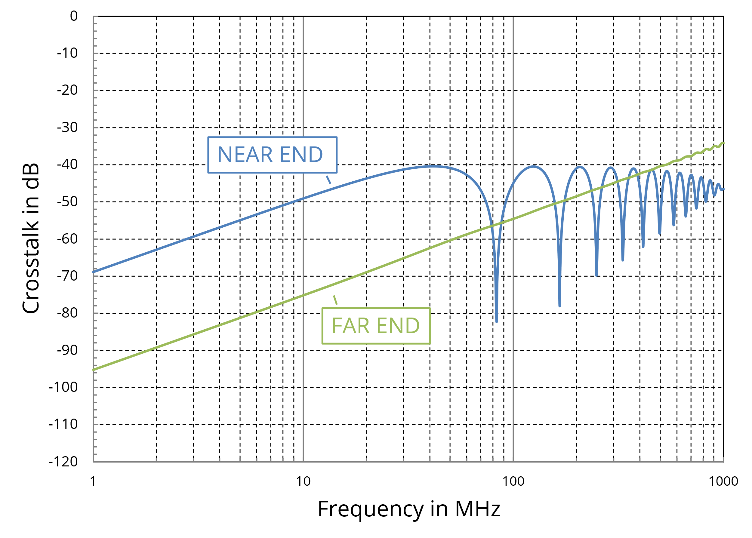
Figure 14. Crosstalk between two lines in non-homogeneous dielectric with C12/(C12+C22) = 0.9 × 10⁻² and L12/L11 = 10-2.
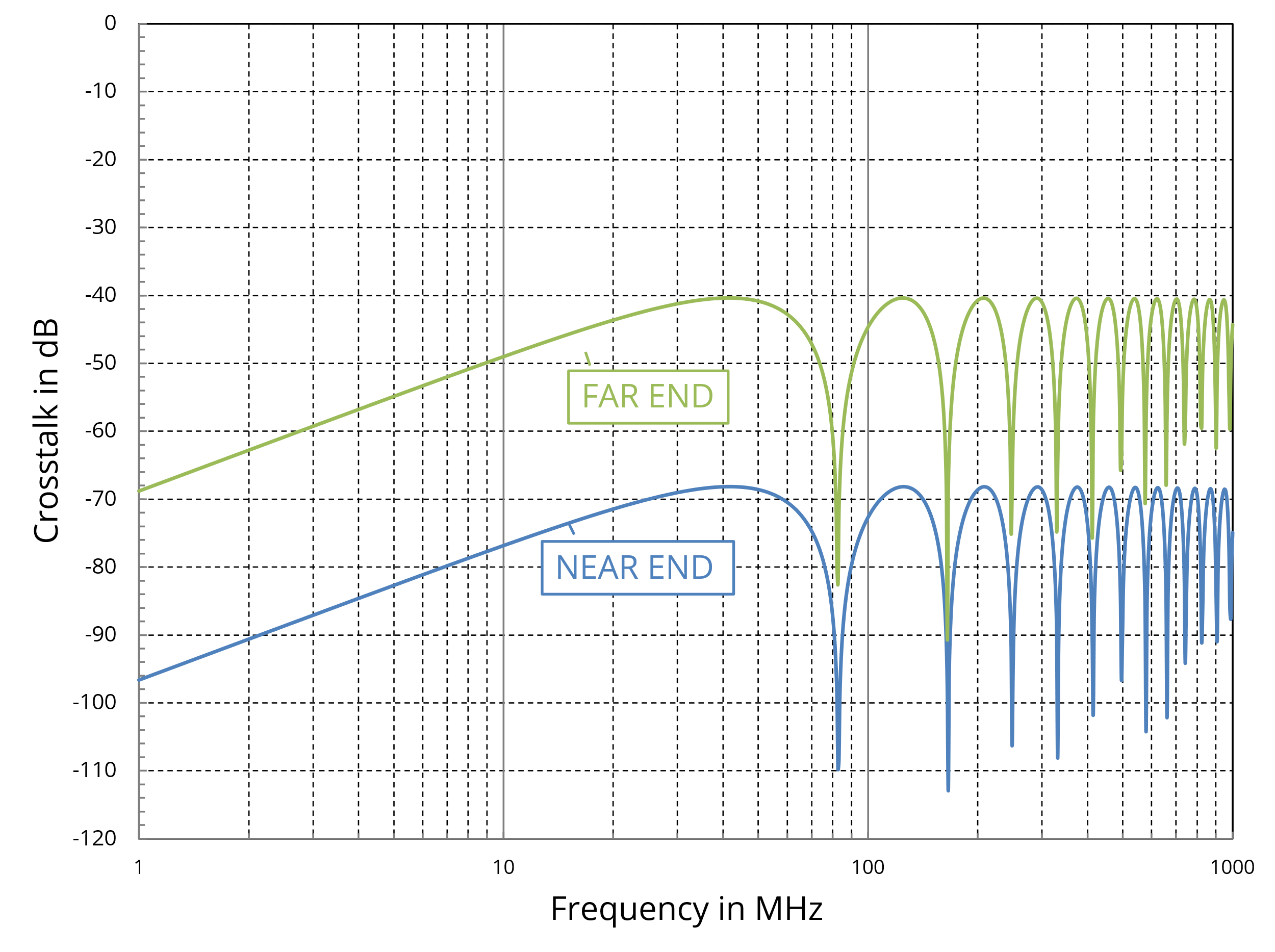
Figure 15. Crosstalk with L12/L11 = 10-2 and RNE2=1 Ω.
Transmission lines are often matched at one end or the other, but not both. Figure 15 shows the calculated crosstalk for the same configuration modeled in Figure 13, except the source resistance of the victim circuit has been changed to 1 Ω. In this case, the coupled power flowing to the near end is reflected and now appears at the far end. When the far-end termination of the source transmission line is set to 5 kΩ, both the near-end and far-end crosstalk are equal, as illustrated in Figure 16.
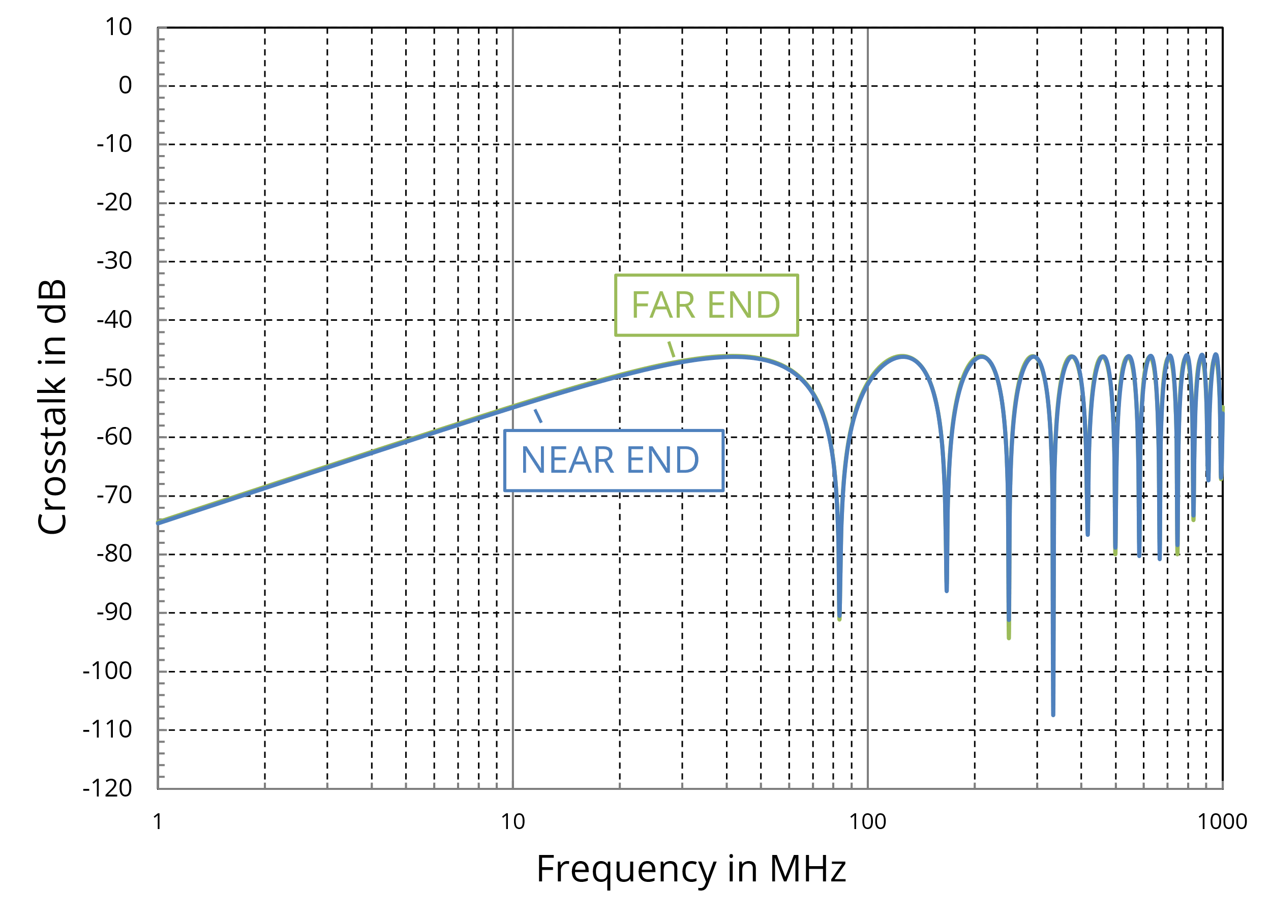
Figure 16. Crosstalk with L12/L11 = 10-2 and RFE1=5 kΩ.
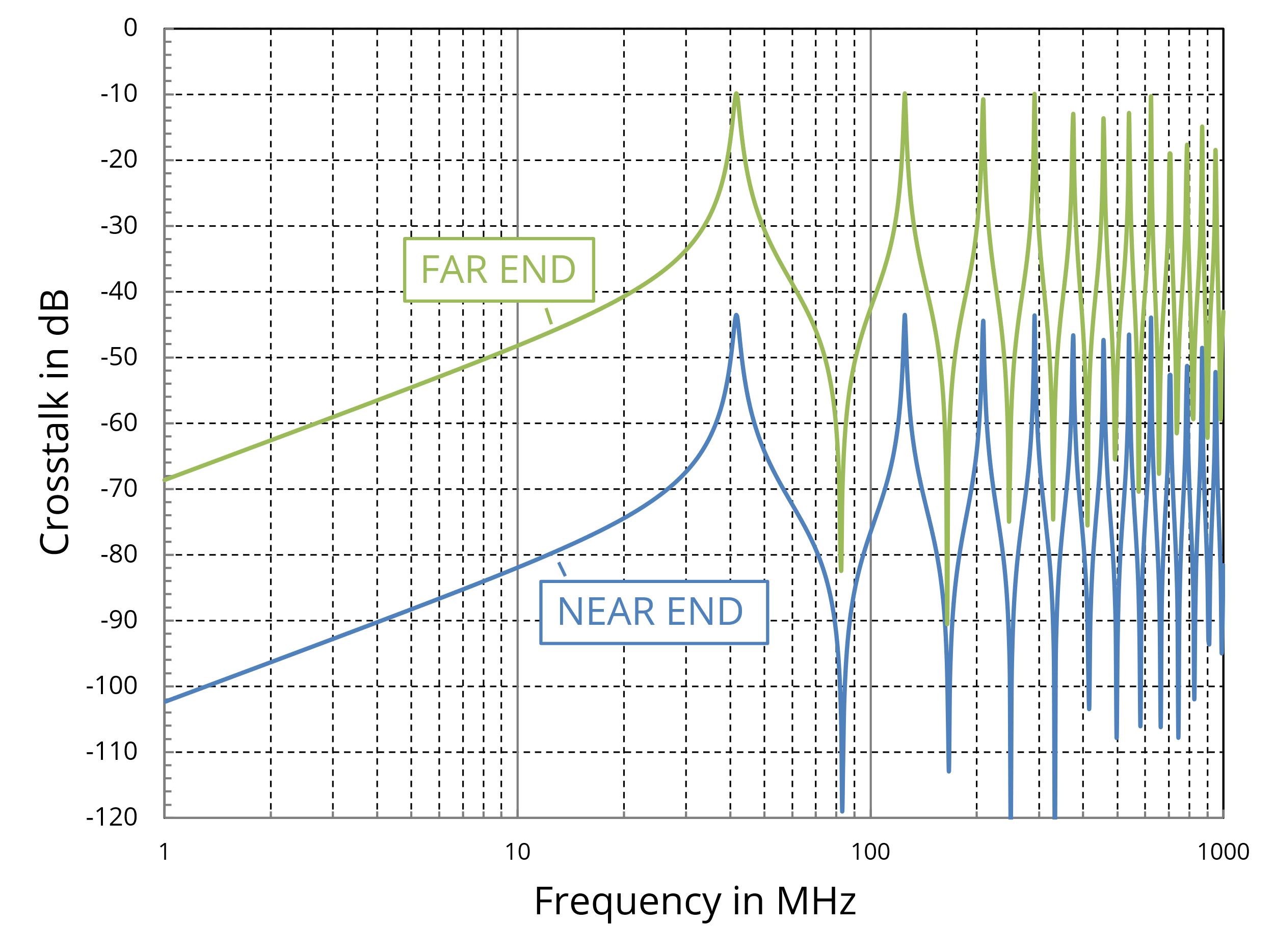
Figure 17. Crosstalk with L12/L11 = 10-2 and RNE2=1 Ω and RFE2=5000 Ω.
And finally, when the near-end termination of the victim line is 1 Ω and the far-end termination is 5 kΩ, the victim line becomes nearly lossless. In this configuration, significant crosstalk is observed at the resonances of the victim transmission line, as illustrated in Figure 17. This result emphasizes the importance of matching a long transmission line at one or both ends.
The same SPICE models used to perform frequency-domain crosstalk calculations can also be used to calculate the coupled voltage in the time domain. For example, exciting the model used to produce the frequency- domain result in Figure 13, with a 1-volt step function produces the time-domain crosstalk shown in Figure 18. In this case, the coupling coefficient is 10-2 and the transition time of the step function is 1 ns. The crosstalk is not specified in decibels, but rather as a simple ratio (i.e., the coupled voltage relative to 1 volt).
Note that the propagation delay is 6 ns. The near-end crosstalk shows up immediately and rises to its peak value of in 1 ns. It remains at that value for twice the propagation delay and then falls back to zero in another 1 ns. The far-end crosstalk is nearly zero because the modeled transmission line is in a homogeneous dielectric (i.e., ).
Figure 19 shows the calculated crosstalk of the same lines when the source resistance of the victim line is changed from 50 Ω to 1 Ω. In this case, most of the near-end coupling is reflected and appears at the far end after 6 ns.
Figure 20 shows the calculated crosstalk when both lines are nominally matched, but the coupling is stronger (L12 / L11 = 0.1). In this case, the coupling is strong enough to alter the characteristic impedance of both lines. The 50-Ω source impedance on the victim line is no longer a perfect match so some of the near-end crosstalk is reflected and appears at the far end.
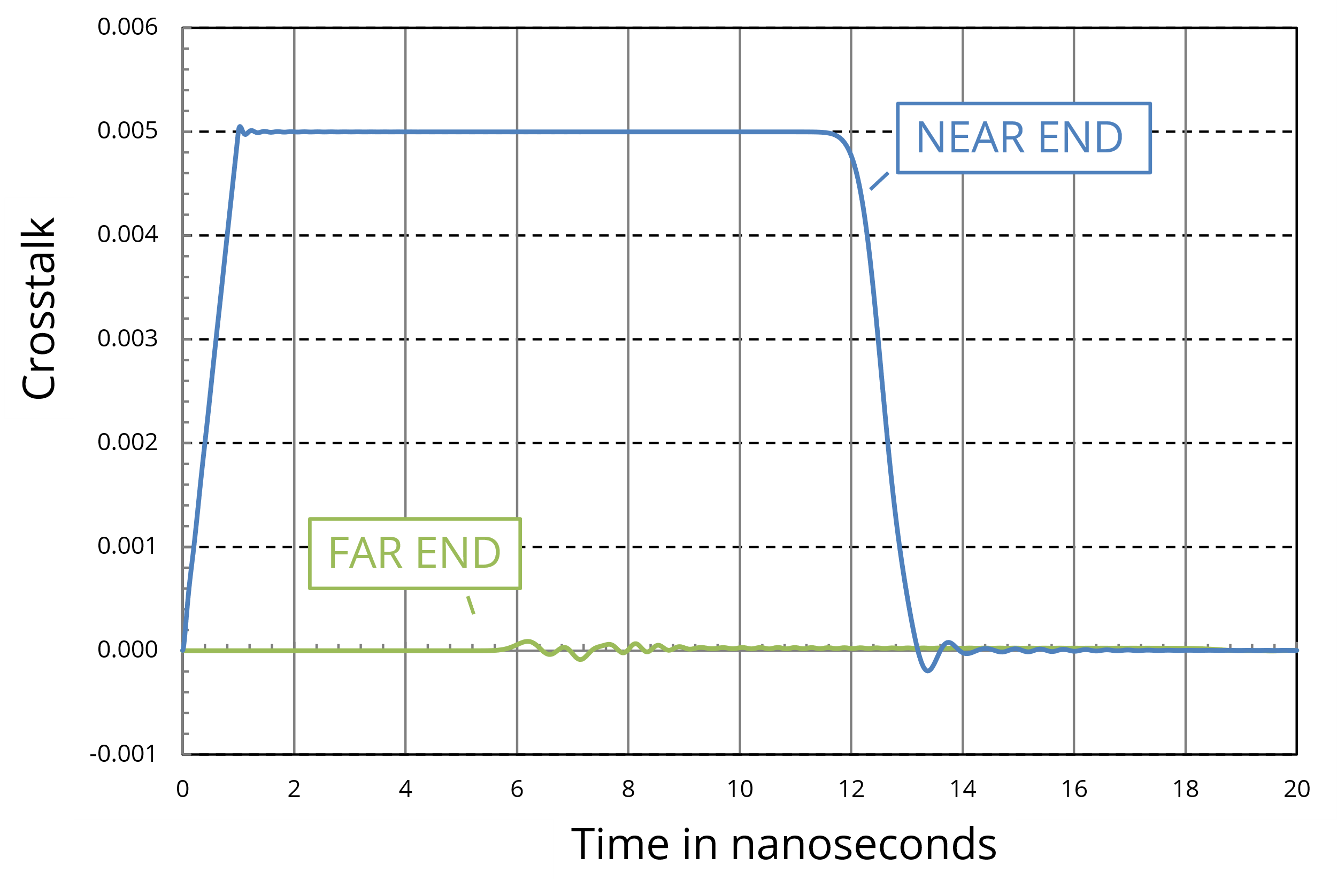
Figure 18. Crosstalk between matched lines with L12/L11 = 10-2.
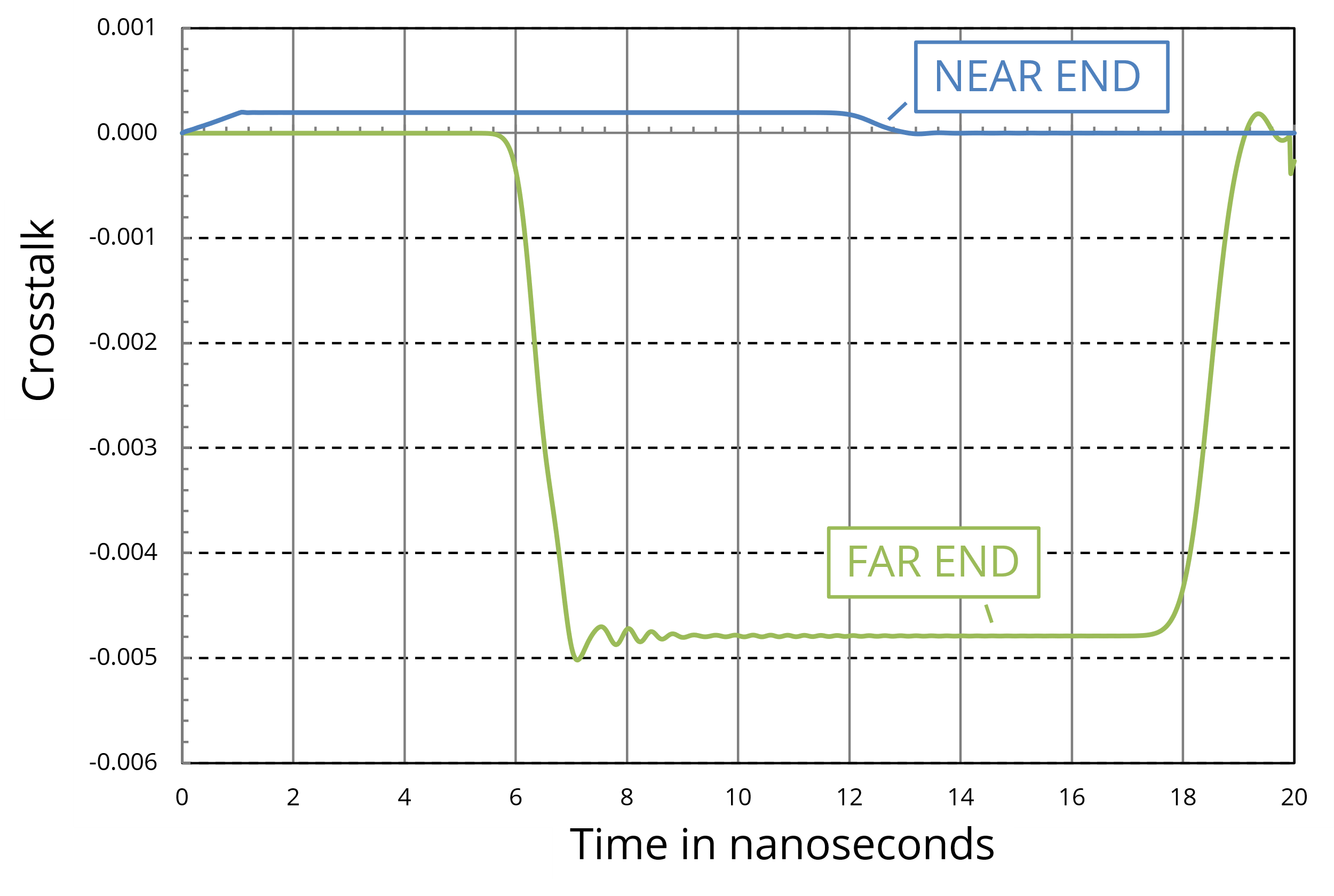
Figure 19. Crosstalk with L12/L11 = 10-2 and RNE2=1 Ω.
Finally, Figure 21 shows the calculated crosstalk when both lines are matched, but the dielectric is nonhomogeneous. In this case, C12 / (C12+C22) = 0.9 × 10‑2, while L12 / L11 = 1.0 × 10‑2. The transmission lines are the same as those whose frequency-domain crosstalk is plotted in Figure 14.
When the dielectric is not homogeneous, the electric-field and magnetic-field coupling do not cancel in the forward direction. In this case, as shown in the figure, a spike is observed at the far end with a peak magnitude nearly as high as the amplitude of the near-end coupling.
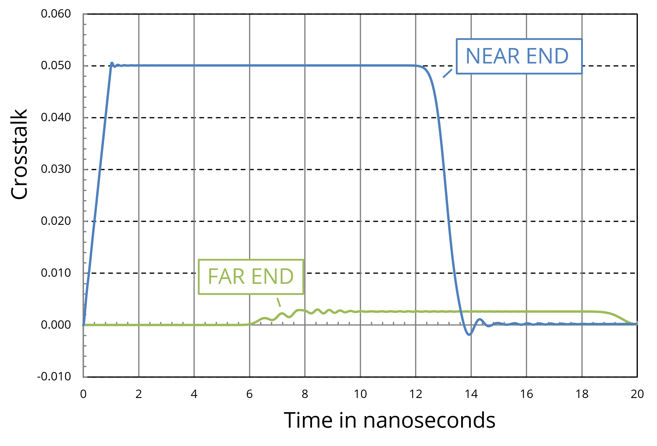
Figure 20. Crosstalk between matched lines with L12/L11 = 10-1.
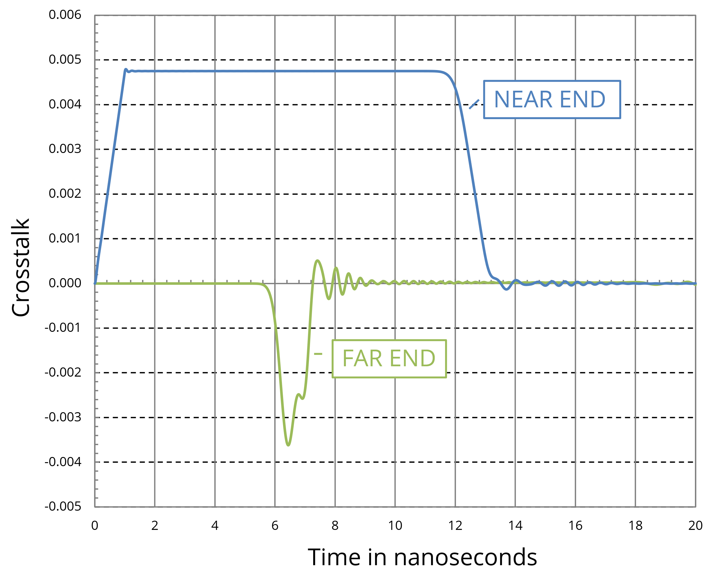
Figure 21. Crosstalk between two lines in non-homogeneous dielectric with C12/(C12+C22) = 0.9 × 10⁻² and L12/L11 = 10-2.
Quiz Question: How would the lumped element model in Figure 11 be different if the ground conductor was the same size and shape as the other two conductors?
There is no inherent assumption that the ground conductor is any different than the signal conductors. In the RLCG model, the ground conductor is simply the zero-volt reference for all other voltages, and all voltage differences are defined only within a given cross-sectional plane of the transmission line. A model similar to the one in Figure 11 can be applied to any three-conductor transmission line, and any of the three conductors can be designated as the ground. Labeling a conductor “ground” impacts how we define our signals, but it does not affect the physics of the coupling.