Although capacitance is essentially a static-field concept, it is fundamental to the description and analysis of both static and time-varying configurations. It is not always important to be able to calculate capacitances precisely, but understanding what capacitance is and estimating the magnitude of self and mutual capacitances are essential skills for any EMC engineer.
Capacitance Between Two Conductors
In a system consisting of two conducting objects, applying a voltage (V) between them would move a charge (Q) from the object at the lower potential to the object at the higher potential. The amount of charge would be directly proportional to the applied voltage, so the ratio of the two quantities would be a constant. This constant is referred to as the mutual capacitance between the two conductors and is given by,
(1)
where V is the electrostatic potential between the two conductors and Q is the magnitude of the equal and opposite charge on the two conductors.
The mutual capacitance is a function of the conductor geometry and the permittivity of the dielectric between them. Lines of electric field start on the conductor with the higher potential and terminate on the conductor with the lower potential. For a given voltage, the mutual capacitance quantifies the total electric flux between the two conductors and plays a vital role in quantifying electric-field coupling.
If the voltage increases in amplitude, the energy stored in the electric flux must also increase. This added energy must come from the source, so the capacitance of a pair of conductors represents an impedance to an increasing voltage. Likewise, if the voltage decreases, energy stored in the electric flux must be returned to the source, which tends to prevent the voltage from decreasing further. Therefore, mutual capacitance is a property that tends to impede changes in the voltage between two conductors.
For simple geometries with a great deal of symmetry, we can calculate the capacitance between the two conductors by placing an equal and opposite charge on each conductor, determining the electric field from the charge distribution, and calculating the voltage by integrating the electric field along a path from one conductor to the other. This works well for large parallel plates, concentric spheres, and concentric cylinders (e.g., as illustrated in Example 1). For most other geometries, the mutual capacitance must be estimated by making comparisons to configurations with a known capacitance or determined precisely using numerical modeling techniques.
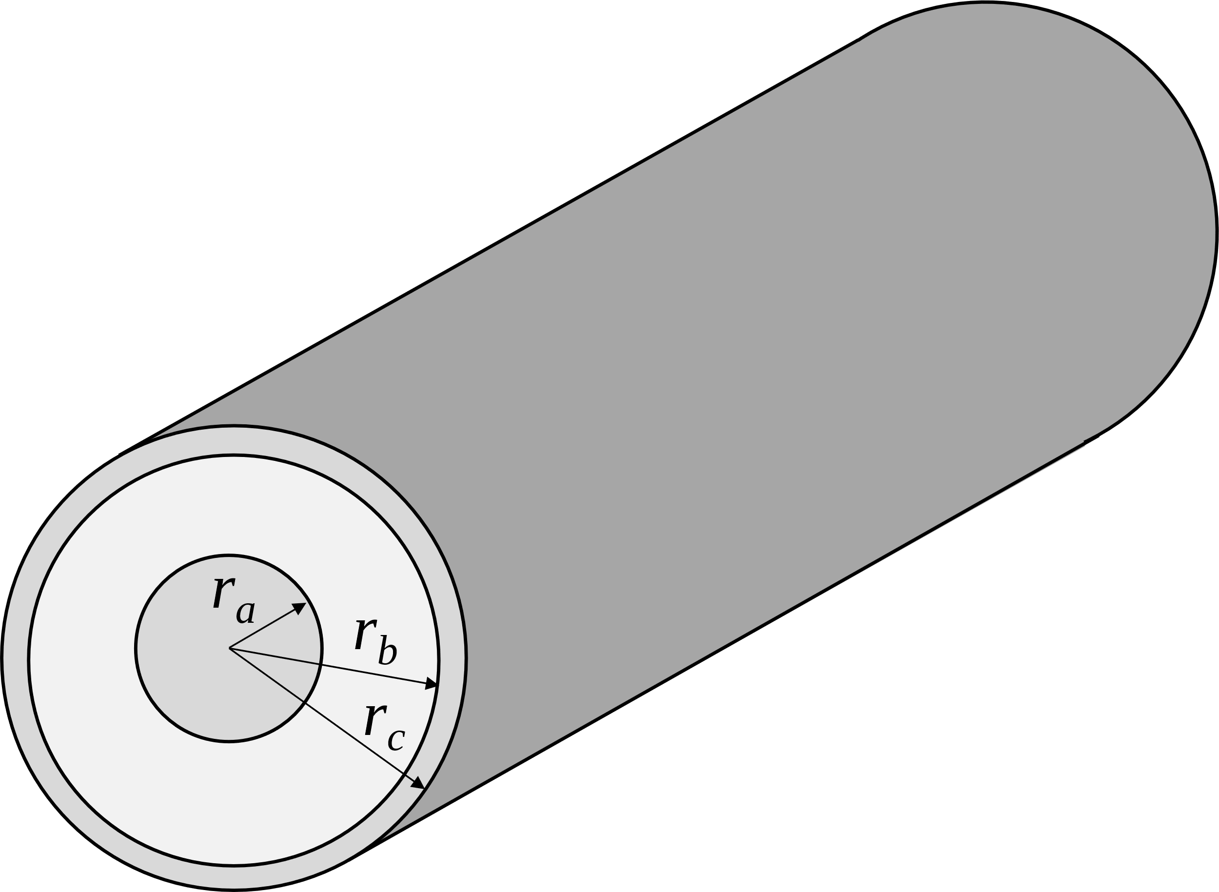
Note that the geometry in Example 1 is that of a coaxial transmission line, so the result shown is the expression for the capacitance per unit length of a coaxial cable. Generally, the mutual capacitance between two objects increases as the distance between them decreases. It will also be proportional to the dielectric permittivity, with the smallest possible permittivity being that of free space, which is ε0 = 8.854 × 10⁻¹² F/m.
Example 1: Capacitance per Unit Length of Coaxial Cable
Find an expression for the capacitance per unit length of the coaxial cable shown in the figure.
By symmetry, the charge density is uniform, so that we can assume a line charge density of ρl coulombs per meter on the inner conductor. Applying Gauss’s Law and taking advantage of the symmetry, the electric field between the cylinders is found to be,
Integrating the electric field from the inner cylinder to the outer cylinder, the potential between the two conductors is,
The capacitance per unit length is the charge per unit length divided by the potential,
Capacitance of One Conductor
While mutual capacitance is an important concept for evaluating conductors in close proximity, absolute capacitance plays an equally important role in EMC engineering. Conductive objects can hold a well-defined amount of charge and take on a well-defined voltage relative to distant objects, even when those distant objects are not well-defined. To illustrate the concept of absolute capacitance, we will start by calculating the mutual capacitance between two concentric spheres as shown in Example 2.
Taking the limit as the radius of the outer sphere gets arbitrarily large, we see that a sphere (or a finite object of any shape) holds a given amount of charge whenever its voltage (relative to infinity) is non-zero. The amount of charge is proportional to the voltage, but independent of the location of other distant conductors.
Absolute capacitance, in general, can be defined as the ratio of the charge on an object relative to its absolute potential. It is a measure of the total charge on an object at a given potential when the conductor is remote from other conductors and charges.
Quiz Question
How much charge does it take to raise a person’s potential to 25,000 volts?
about 1 coulomb
a few microcoulombs
a few picocoulombs
Example 2: Concentric Conducting Spheres
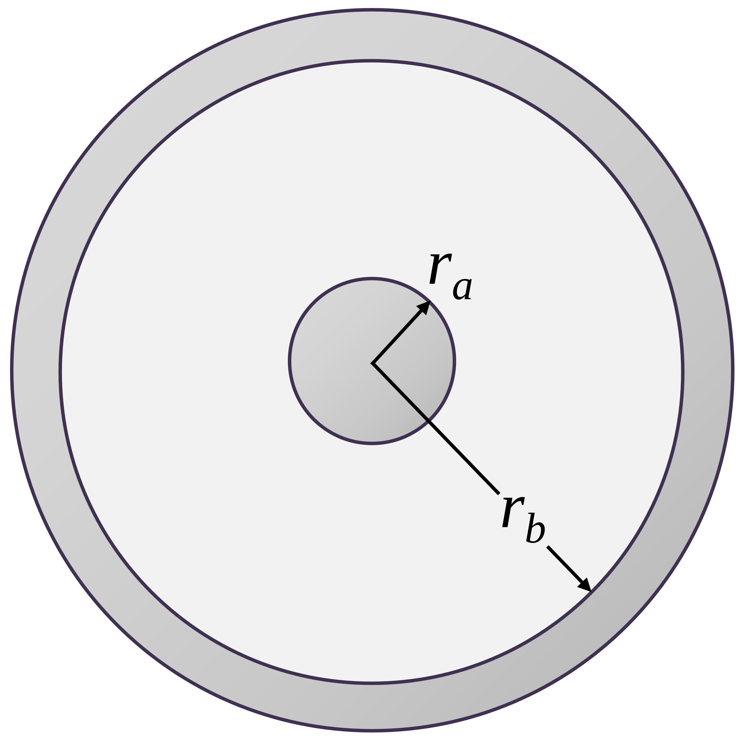
Determine the capacitance between the two conductive spheres illustrated on the right.
If the charge on the inner sphere is Q0 coulombs, then the electric field between the spheres can be determined by applying Gauss’s Law and taking advantage of the structure symmetry,
The voltage between the spheres is found by integrating the electric field,
and the capacitance is then shown to be,
Note that as the radius of the outer sphere approaches infinity, the capacitance does not approach zero. An absolute capacitance can be defined for the inner sphere as,
The voltage difference, Vab, also takes on a fixed, finite value as rbgoes to infinity. This is the absolute potential of the sphere, or its voltage relative to infinity. However, because the electric field drops off rapidly at distances much larger than the inner sphere diameter, the absolute potential is essentially the voltage difference between the sphere and uncharged objects that are not located nearby.
This is an important concept for EMC engineers because it illustrates how any conducting object can become charged even when it is not near another conducting object. For example, a person dragging their rubber-soled shoes across a wool carpet on a dry day can become charged to ~25,000 volts. The amount of charge they carry depends on their absolute capacitance, Qstored = Cabs × 25,000 volts.
A person curled up in a ball with a radius of about 0.5 meters will have an absolute capacitance of about Cabs = 4πε0ra ≈ 60 pF. If the person stands erect, their absolute capacitance will be higher (e.g., 100 pF), because the charge can spread out more. A 100-pF person charged to 25,000 volts will hold approximately Q = (100 × 1012 F) (25,000 V) = 2.5 µC of charge.
Self and Mutual Capacitance
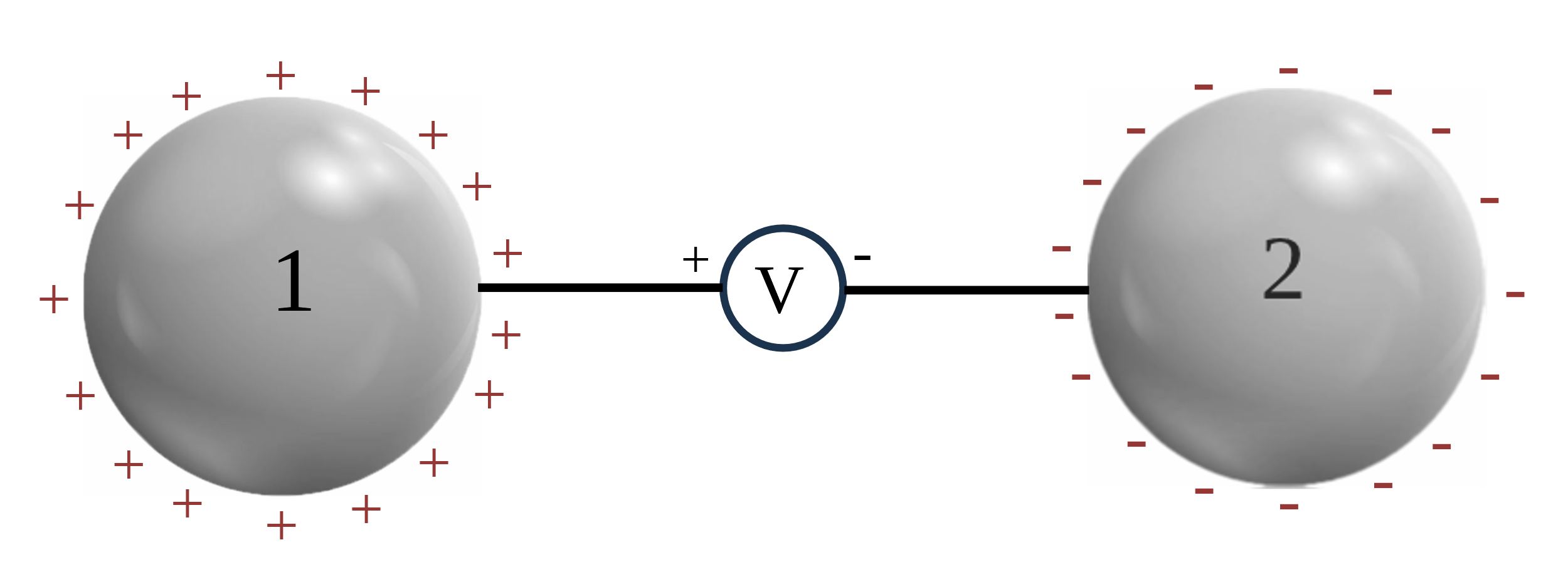
Figure 1. Two spheres with an applied voltage between them.
It can be helpful to view absolute capacitance as a capacitance to infinity. Lines of electric field originating from the object terminate infinitely far away. In the real world, if we place charge on an object, it is always drawn from somewhere else. So, let’s consider the case where charge is pulled from one sphere and put on another nearby sphere, as illustrated in Figure 1. There is a positive charge, Q, on one sphere and an equal negative charge on the other. The ratio of the charge to the voltage between the spheres is the mutual capacitance between the spheres.
When the spheres are very close, the capacitance between the spheres is relatively high. This capacitance decreases as the spheres are moved farther apart, but there is a limit to how small the capacitance can become. Each sphere has a capacitance to infinity, so no matter where the spheres are located, each sphere will always hold a charge proportional to its absolute voltage.
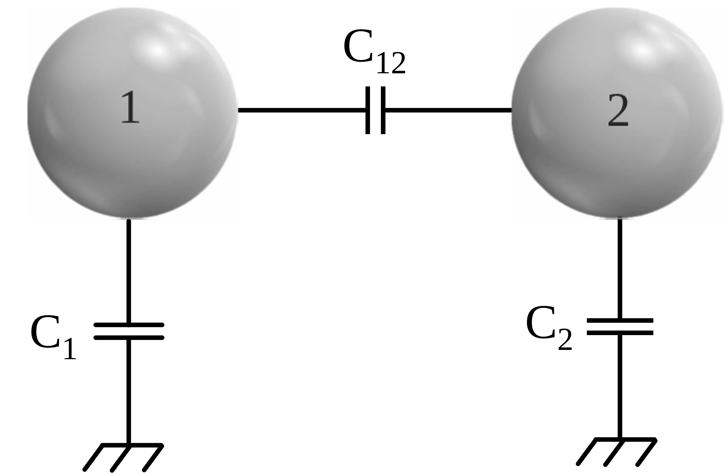
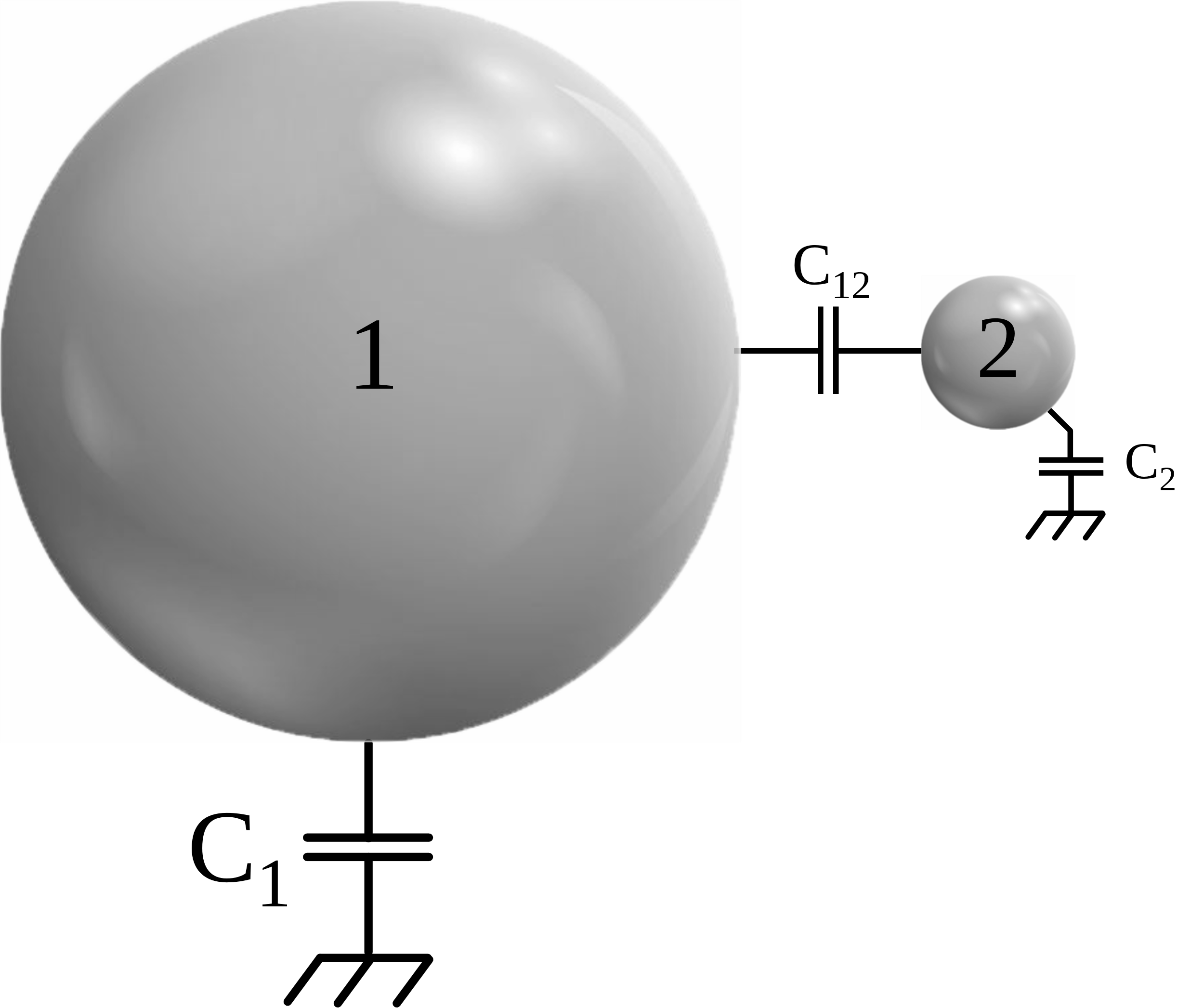
Schematically, we can model this system with three capacitances as illustrated in Figure 2. In the model, the voltage at infinity is zero, so lines of electric flux that terminate at infinity are modeled as a self-capacitance to the zero-volt reference (electrical ground). Lines of flux originating on one sphere and terminating on the other sphere are represented by the partial mutual capacitance, C12.1 If the capacitance between the two spheres were measured, we would expect the measured value to be,
(2)
The flux flows through C12 or the series combination of C1 and C2.
Figure 2. Schematic representation of self and partial mutual capacitances.
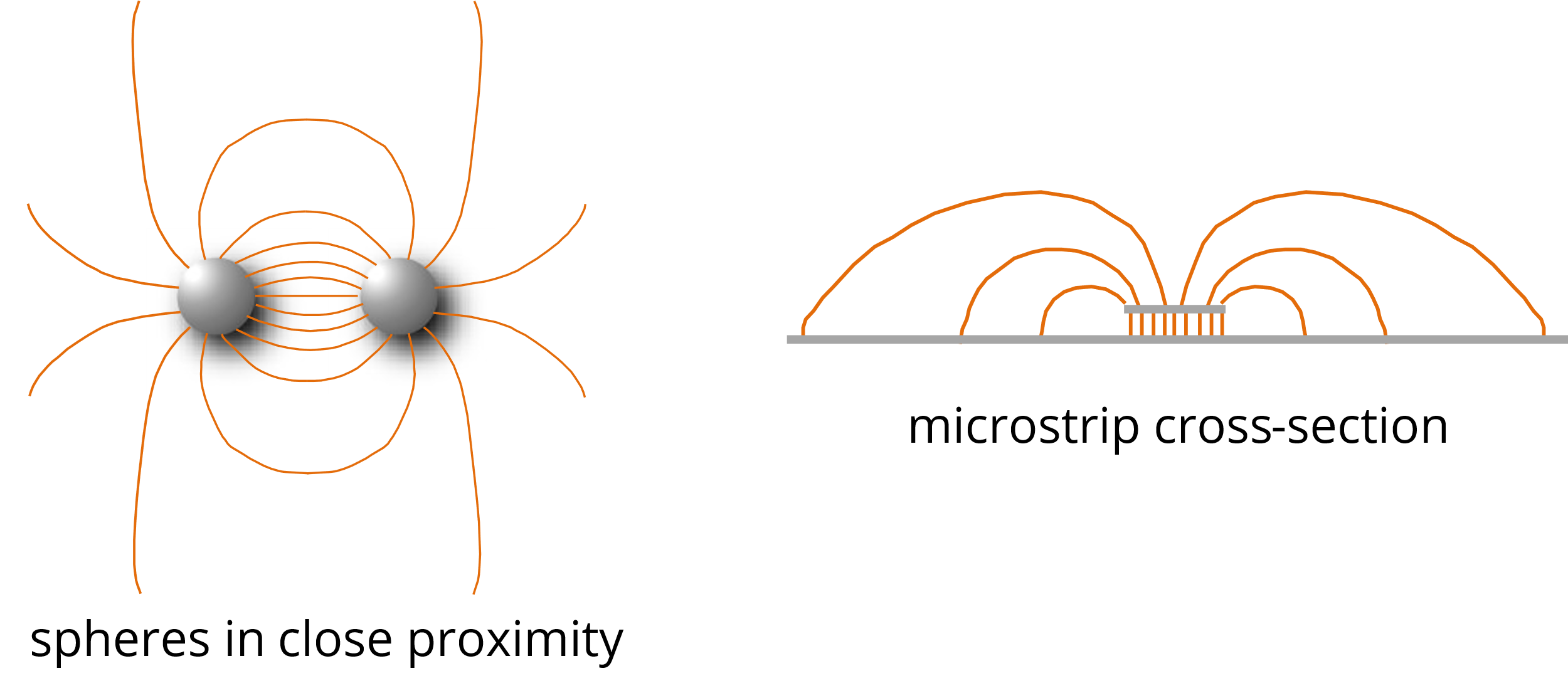
If the spheres are very close to each other relative to their diameter, most of the electric flux is concentrated in short lines that start on one sphere and terminate on the other sphere. The flux extending far from the immediate vicinity of the spheres is relatively weak. In this case, the value of C12 is relatively high while the values of C1 and C2 are small.
As the spheres are moved farther apart, the value of C12 decreases. Less of the flux emanating from one sphere is immediately captured by the other sphere. More of the flux extends far from the system where the relative position of the two spheres is unimportant, so the values of C1 and C2 increase. Once the distance between the two spheres is great enough (e.g., 5-10 sphere diameters), C1 and C2 are approximately equal to the absolute capacitances of their respective spheres. The value of C12 decreases to the point where it is much smaller than the series combination of C1 and C2. At this point, the distance between the two spheres no longer significantly affects their measured mutual capacitance.
Now let’s examine what happens when the diameter of one sphere is significantly increased while maintaining an edge-to-edge separation larger than the smaller sphere’s diameter. For example, as the sphere on the left in Figure 2 grows, as illustrated in Figure 3, the value of C1 gets larger. C12 also increases slightly, while C2 decreases. The larger sphere captures more lines of flux emanating from the smaller sphere, and fewer lines extend to infinity.
In the limit as the first sphere grows infinitely large, C1 becomes infinite, and the first sphere becomes the zero-volt reference. At the same time, C2 goes to zero. All the flux from sphere 2 is captured by sphere 1. However, as long as the distance between sphere 1 and sphere 2 is much greater than the diameter of sphere 2, the total flux emanating from sphere 2 (for a given voltage) is the same. The value of C12 approaches the absolute capacitance of C2. In other words, when one conductor is much larger than the other, the mutual capacitance between them depends only on the size and location of the smaller conductor. And if the distance between the two conductors is large compared to the size of the smaller conductor, the mutual capacitance is essentially equal to the absolute capacitance of the smaller conductor.
Figure 3. Schematic representation of self and partial mutual capacitances in spheres of different sizes.
For example, suppose the larger sphere is the Earth (diameter ~12,800 km) and the smaller sphere is a soccer ball (diameter ~22 cm). Suppose the soccer ball is 1 meter above the ground. Strictly speaking, the soccer ball’s capacitance to infinity is zero; however, its capacitance to the earth is equal to its absolute capacitance. In other words, the soccer ball holds the same amount of charge for a given voltage whether or not the Earth is present.
In the literature, the term capacitance to earth is sometimes used to describe an absolute capacitance. Technically, this is correct if the conducting object is anywhere within a few thousand kilometers of the Earth. Nevertheless, the term can be confusing because it implies that the presence of the earth has something to do with the value of this capacitance.
In electronic systems, any conducting object with an absolute capacitance much larger than the other objects in the system can replace infinity or the earth as the zero-volt reference. In many systems, a metal chassis or enclosure serves this purpose.
Capacitance in a System of Conductors
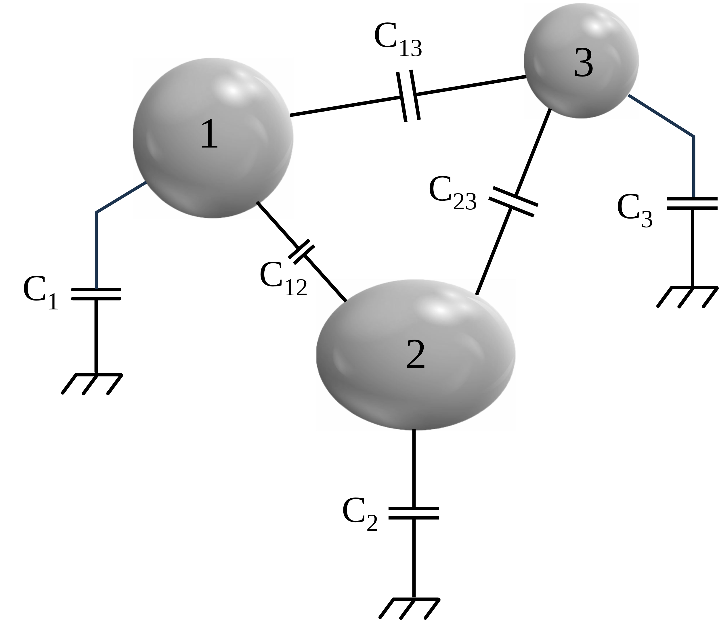
If we have several conductive objects, we can define a self-capacitance value for each conductor and a partial mutual capacitance2 between each conductor pair. Figure 4 illustrates this for a system of 3 conductors. The superposition principle is applied to calculate these self and mutual capacitances. The absolute potential of each conductor can be expressed as the sum of the potentials due to charge on each of the other conductors and its own charge.
Figure 4. Self and Mutual Capacitance.
For n conductors,
(3)
volts
where the coefficients of potential, pij, are functions of the geometry. This equation can be written in matrix form as,
(4)
.
Solving this system of equations for Q results in an expression of the form,
(5)
where [c] = [p]-1 is the generalized capacitance matrix. Coefficients of the form cii represent the capacity of the ith conductor. The capacity of a single conductor in a system of conductors is the total charge on the conductor when it is maintained at unit potential and all other conductors are held at zero potential. Coefficients of the form cij, where i ≠ j are referred to as coefficients of induction. These coefficients are always negative or zero and satisfy the relation cij=cji. They represent the ratio of the charge on the ith conductor to the absolute potential of the jth conductor when all conductors except the jth conductor are at zero potential. Self and mutual capacitance values, which are always non-negative, can be calculated from the elements of the generalized capacitance matrix using the relations,
(6)
Once these values have been calculated for a system of conductors (e.g., Figure 4), the behavior of the system can be analyzed using simple circuit modeling techniques.
Example 3: Capacitance of Power Lines
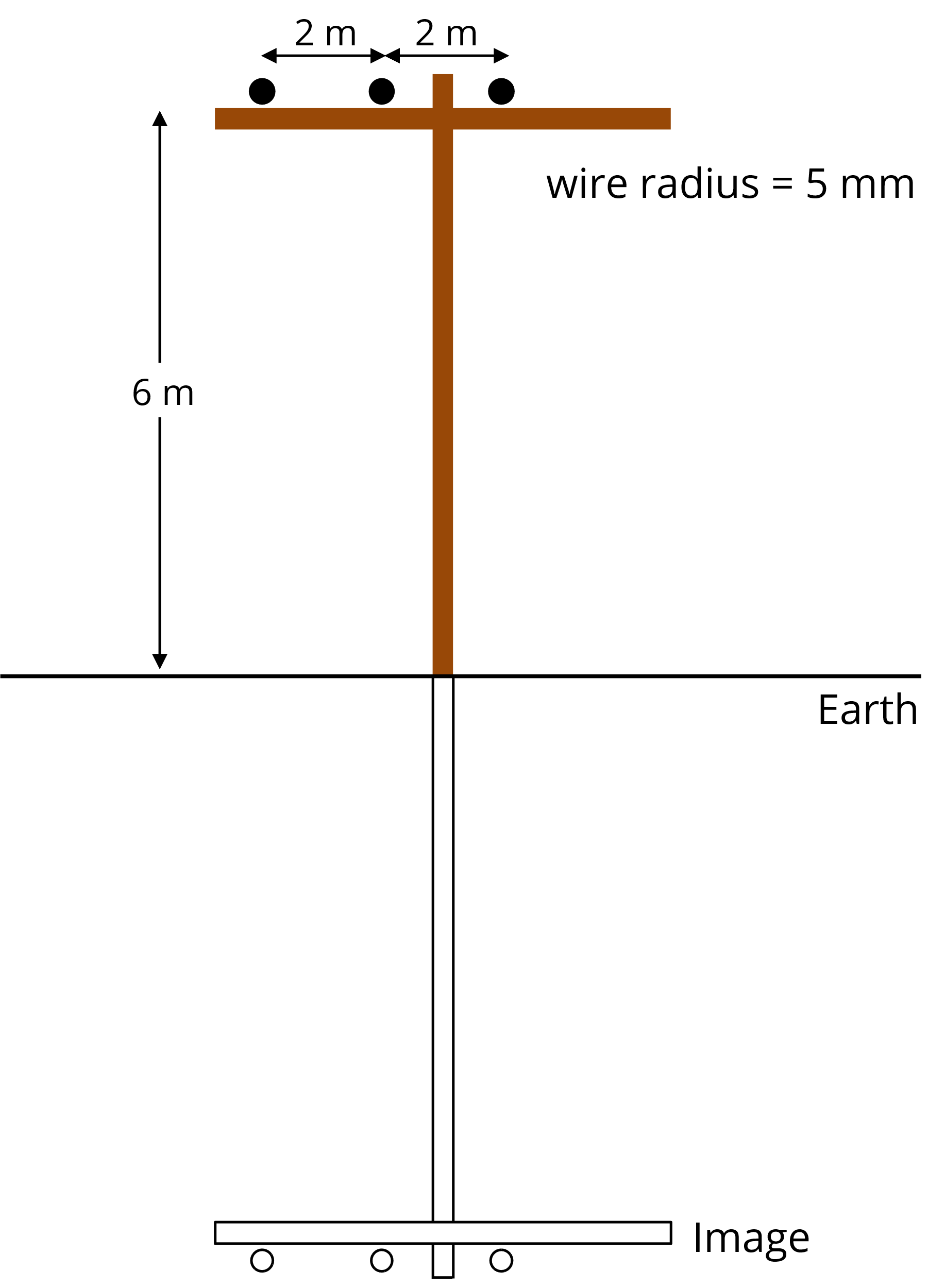
Determine the self and mutual capacitances between three power lines mounted on a pole 6 meters above the ground. The wires are lined up horizontally with a 2meter spacing. The wire radius is a = 5 mm.
Each wire is represented by a line charge at the wire’s center. The potential between two points at distances r1 and r2 from the uniform line charge is,
where q is the magnitude of the line charge in coulombs per meter. If r1 is set to the wire’s radius, a, and r2 is set to twice the distance of the wire above ground, h, the potential on the surface of theith wire due to the wire’s own charge and its image in the ground plane is,
where pii is a coefficient relating charge to potential as defined in (3). The potential on the jth wire due to the charge on theith wire is readily shown to be,
where dij is the distance between the ith and jth wire and d'ij is the distance between the ith wire and the image of the jth wire.
Using the dimensions given in the figure, the following values are calculated,
Putting these results in matrix form gives,
.
Inverting the matrix results in the following values for the generalized capacitance matrix,
.
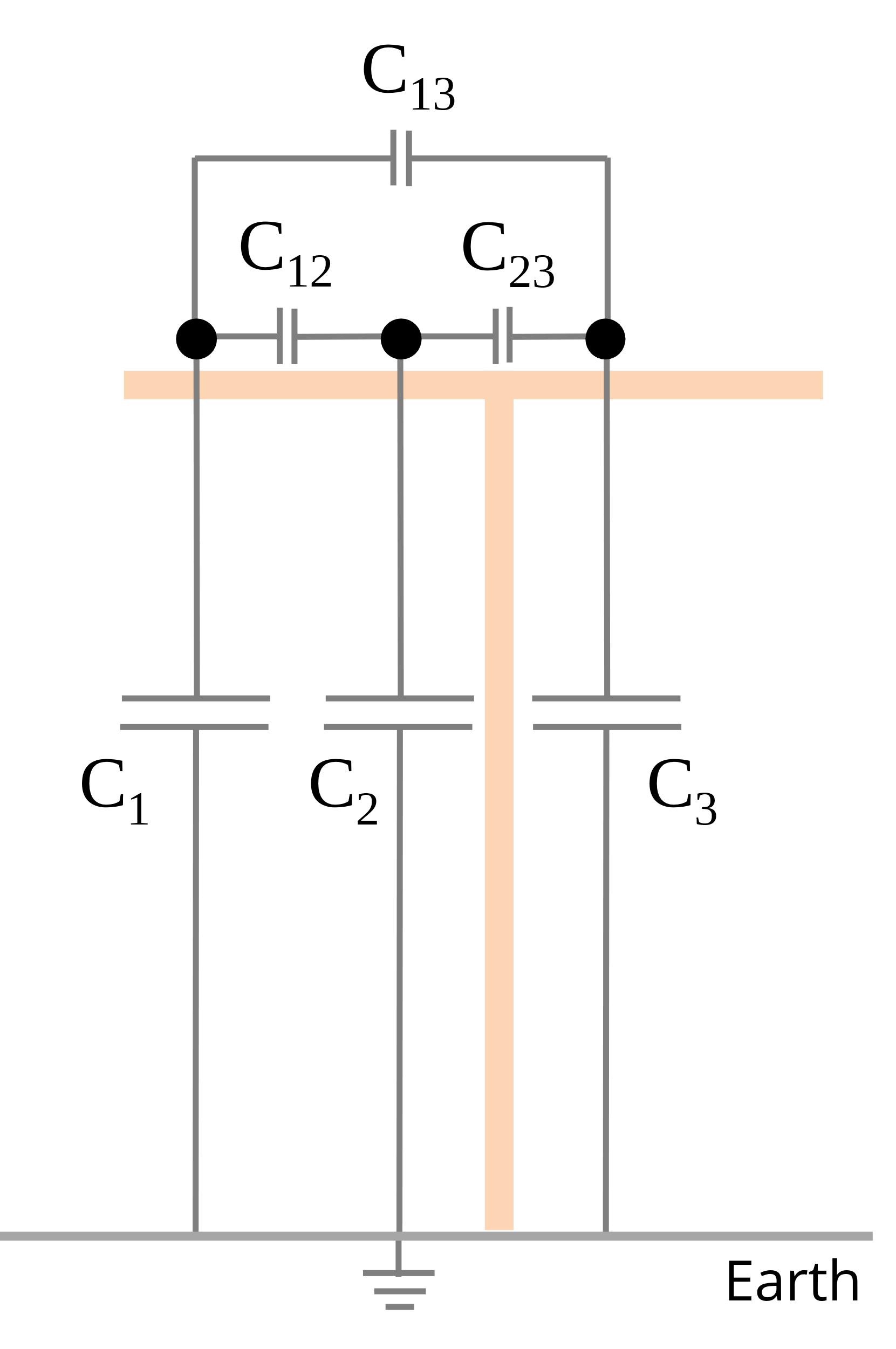
We can then solve for the mutual capacitance between each wire and the wire-to-ground capacitances.
These values can be used to calculate the capacitive coupling between the power lines using the equivalent circuit illustrated on the right.
In this example, the charge was uniformly distributed on the wire. However, when conductive objects are in close proximity, such as wires in a cable bundle or printed circuit board traces, charge may be concentrated on certain parts of the conductors, as illustrated by the concentration of electric flux lines in Figure 5.
Figure 5. Geometries with non-uniform charge distributions.
Example 4: Coupling Between Shielded Conductors
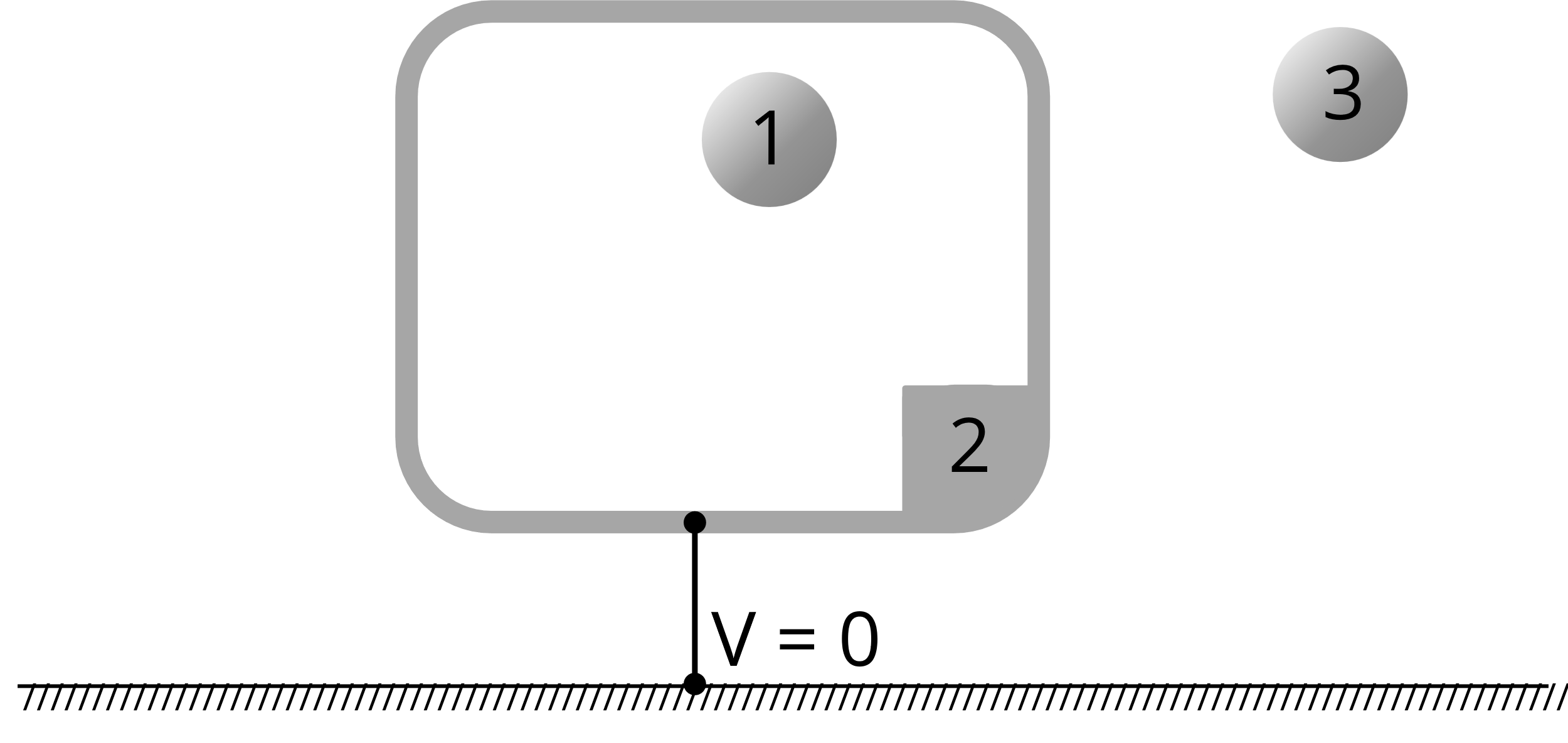
Suppose a conductive object is surrounded by another conductor, as illustrated below. The charge and absolute potential of this configuration are related by the system of equations,
where V2 is our reference potential and was set to zero.
In the special case where q1 = 0, the potential V1 also must be zero because the potential everywhere inside a closed, equipotential surface without enclosed sources must equal the potential on the surface. Setting q1 and V1 equal to zero in the equation above indicates that,
which must be valid for any value of V3. Therefore, c13 must be zero.
Although this value was derived by setting q1 = 0, the coefficients of induction are functions of the geometry only. Therefore, c13 = C13 = 0 even if there is charge on the first conductor. In other words, a charge on the first conductor does not affect the potential of the third conductor. Also, because the capacitance matrix is symmetric, c31= C31 = 0, and a charge on the outer conductor cannot affect the potential of the inner conductor.
The #2 conductor is an electrostatic shield. Static electric field and charge distributions outside the shield are entirely independent of those inside the shield. This principle is often used to protect sensitive devices from strong external fields or to contain the fields of undesired sources.
In these cases, an accurate closed-form expression relating potential to the charge on the conductors may not be obtainable. Nevertheless, the problem can be solved by dividing each conductor into a system of smaller conductors, each with an approximately uniform charge distribution. The self and mutual capacitances of each “piece” can then be calculated, and the results recombined to get the self and mutual capacitances of the larger objects. This technique is efficient, accurate and relatively easy to apply using static field solvers. The concept of breaking a large problem into a system of smaller problems is very powerful. A variety of numerical electromagnetic modeling and analysis tools employ this general approach.
While the definition of capacitance depends on the concept of electrostatic potential, values of capacitance are primarily a function of the geometry. Therefore, capacitance also has meaning in time-varying situations, provided the conductive surfaces are small enough to ensure that they have a uniform potential. Generally, this condition is satisfied when all surface dimensions are much smaller than the shortest wavelength of interest.
Notes
Note that for two spheres in the middle of an empty universe, all lines of flux originating on one sphere eventually terminate on the other. The term partial mutual capacitance is introduced to represent the part of the mutual capacitance that approaches zero as the distance between the spheres is increased. ↩
The term partial mutual capacitance was introduced to distinguish it from the term mutual capacitance as defined for a two-conductor system. However, in systems of conductors, the word partial is commonly dropped. Through the rest of this chapter the term mutual capacitance will refer to the partial mutual capacitance in a system of conductors. The term effective capacitance will be used to describe the capacitance between two conductors due to all available flux paths. ↩